From award-winning research demos to photorealistic graphics created with NVIDIA RTX and Omniverse, see how NVIDIA is breaking boundaries in AI, graphics, and virtual collaboration.
It’s one thing to hear about something new, amazing, or downright mind-blowing. It’s a completely different experience when you can see those breakthroughs visualized and demonstrated. At SIGGRAPH 2021, NVIDIA introduced new and stunning demos showcasing how the latest technologies are transforming workflows across industries.
From award-winning research demos to photorealistic graphics created with NVIDIA RTX and Omniverse, see how NVIDIA is breaking boundaries in AI, graphics, and virtual collaboration.
Watch some of the exciting demos featured at SIGGRAPH:
Real-Time Live! Demo: I AM AI: AI-Driven Digital Avatar Made Easy
This demo won the Best in Show award at SIGGRAPH. It showcases the latest AI tools that can generate digital avatars from a single photo, animate avatars with natural 3D facial motion, and convert text to speech.
Interactive Volumes with NanoVDB in Blender Cycles
See how NanoVDB makes volume rendering more GPU memory-efficient, so larger and more complex scenes can be interactively adjusted and rendered with NVIDIA RTX-accelerated ray tracing and AI denoising.
Interactive Visualization of Galactic Winds with NVIDIA Omniverse
Learn more about NVIDIA IndeX, a volumetric visualization tool for researchers to visualize large scientific datasets interactively, for deeper insights. With Omniverse, users can virtually collaborate in real time, from any location, while using multiple apps simultaneously.
Accelerating AI in Photoshop Neural Filters with NVIDIA RTX A2000
Watch how AI-enhanced Neural Filter in Adobe Photoshop accelerated with NVIDIA RTX A2000 takes photo editing to the next level. Combining NVIDIA RTX A2000 with Photoshop AI, tools like Skin Smoothing and Smart Portrait give photo editors the power of AI for creating stunning portraits.
Multiple Artists, One Server
Discover how to accelerate visual effects production with the NVIDIA EGX Platform, which enables multiple artists to work together on a powerful, secure server from anywhere.
Visit the SIGGRAPH page to watch all the newest demos, catch up on the latest announcements, and explore on-demand content.
Sign up for webinars with NVIDIA experts and Metropolis partners on Sept. 22, featuring developer SDKs, GPUs, go-to-market opportunities, and more.
Join NVIDIA experts and Metropolis partners on Sept. 22 for webinars exploring developer SDKs, GPUs, go-to-market opportunities, and more. All three sessions, each with unique speakers and content, will be recorded and will be available for on-demand viewing later.
Session 1: NVIDIA Fleet Command | Best Practices for Vision AI Development
Wednesday, September 22, 2021, 1 PM PDT
Learn how to securely deploy, manage, and scale your AI applications with NVIDIA Fleet Command.
Hear from Data Monsters, a solution development partner, on how they use Metropolis to solve some of the world’s most challenging Vision AI problems.
Session 2: NVIDIA Ampere GPUs | Synthetic Data to Accelerate AI Training
Wednesday, September 22, 2021, 4 PM CEST
Explore how the latest NVIDIA Ampere GPUs significantly reduce deployment costs and provide more flexible vision AI app options.
No data, no problem! Our synthetic data partner, SKY ENGINE AI, shows how to use synthetic data to fast-track your AI development.
Session 3: NVIDIA Pre-Trained Models | Go-To-Market Opportunities with Dell
Wednesday, September 22, 2021, 1 PM JST
Learn how the Dell OEM team can help bring your Metropolis solutions to market faster.
Go from zero to world-class AI in days with NVIDIA pretrained models. NVIDIA experts will show how to use the PeopleNet model to build an application in minutes and harness TAO Toolkit to adapt the application to different environments.
Learn how the use of RAPIDS to accelerate the analysis of single-cell RNA-sequence on a single NVIDIA V100 GPU shows a massive performance increase.
Single-cell genomics research continues to advance drug discovery for disease prevention. For example, it has been pivotal in developing treatments for the current COVID-19 pandemic, identifying cells susceptible to infection, and revealing changes in the immune systems of infected patients. However, with the growing availability of large-scale single-cell datasets, it’s clear that computing inefficiencies are significantly impacting the speed at which science is done. Offloading these compute bottlenecks to the GPU has demonstrated intriguing results.
In a recent blog post, NVIDIA benchmarked the analysis on one million mouse brain cells sequenced by 10X Genomics. Results demonstrated that the end-to-end workflow took over three hours to run on a GCP CPU instance while the entire dataset was processed in 11 minutes on a single NVIDIA V100 GPU. In addition, running the RAPIDS analysis on the GCP GPU instance also costs 3x less than the CPU version. Read the blog here.
Follow this Jupyter notebook for RAPIDS analysis of this dataset. For the notebook to run, the files rapids_scanpy_funcs.py and utils.py must be in the same folder as the notebook. We provide a second notebook with the CPU version of this analysis here. In collaboration with the Google Dataproc team, we’ve built out a getting started guide to help developers run this trascriptomics use case quickly. Finally, check out this NVIDIA and Google Cloud co-authored blog post that showcases the impact of the work.
Performing single-cell RNA analysis on the GPU
A typical workflow to perform single-cell analysis often begins with a matrix that maps the counts of each gene script measured in each cell. Preprocessing steps are performed to filter out noise, and the data are normalized to obtain expressions of every gene measured in every individual cell of the dataset. Machine learning is also commonly used in this step to correct unwanted artifacts from data collection. The number of genes can often be quite large, which can create many different variations and add a lot of noise when computing similarities between the cells. Feature selection and dimensionality reduction decrease this noise before identifying and visualizing clusters of cells with similar gene expression. The transcript expression of these cell clusters can also be compared to understand why different types of cells behave and respond differently.
Figure 1: Pipeline showing the steps in the analysis of single-cell RNA sequencing data. Starting from a matrix of gene activity in every cell, RAPIDS libraries can be used to convert the matrix into gene expressions, cluster and lay the cells out for visualization, and aid in analyzing genes with different activity across clusters.
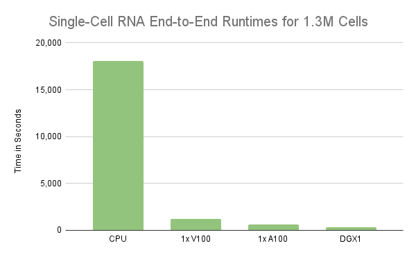
The analysis demonstrates the use of RAPIDS to accelerate the analysis of single-cell RNA-sequence data from 1 million cells using a single GPU. However, the experiment only processed the first 1M cells, not the entire 1.3M cells. As a result, processing all 1.3M cells in a workflow for single-cell RNA data took almost twice the time on a single V100 GPU. On the other hand, the same workflow took only 11 minutes on a single NVIDIA A100 40GB GPU. Unfortunately, the nearly 2x degradation in performance on the V100 is due mainly to the ability to oversubscribe the GPU’s memory so that it spills to host memory when needed. We will cover this behavior in more detail in the following section, but what’s clear is that the GPU’s memory is a limiting factor to scale. So, processing larger workloads faster requires beefier GPUs like the A100 or/and spreading the processing over multiple GPUs.
Benefits of scaling preprocessing to multiple GPUs
When a workflow’s memory usage grows beyond the capacity of a single GPU, unified virtual memory (UVM) can be used to oversubscribe the GPU and automatically spill to main memory. This approach can be advantageous during the exploratory data analysis process because moderate oversubscription ratios can eliminate the need to rerun a workflow when the GPU runs out of memory.
However, relying strictly on UVM to oversubscribe a GPU’s memory by 2x or more can lead to poor performance. Even worse, it can cause the execution to hang indefinitely when any single computation requires more memory than is available on the GPU. Spreading computation across multiple GPUs affords the benefit of both increased parallelism and reduced memory footprint on each GPU. In some cases, it may eliminate the need for oversubscription. Figure 2 demonstrates that we can achieve linear scaling by spreading the preprocessing computations across multiple GPUs, with 8 GPUs resulting in slightly over 8x speedup compared to a single NVIDIA V100 GPU. Putting that into perspective, it takes less than 2 minutes to reduce the dataset of 1.3M cells and 18k genes down to approximately 1.29M cells and the 4k most highly variable genes on 8 GPUs. That’s over an 8.55x speedup as a single V100 took over 16 minutes to run the same preprocessing steps.
Figure 2: Comparison of runtime in seconds for a typical single-cell RNA workflow on 1.3M mouse brain cells with different hardware configurations. Performing these computations on the GPU shows a massive performance increase.
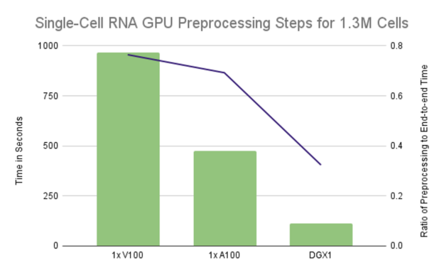
Figure 3: The runtimes of the single GPU configurations are dominated by the preprocessing steps, taking over 75% of the end-to-end runtime on a single V100 and 70% of the runtime on a single A100. Utilizing all of the GPUs on a DGX1 lowers the ratio to just over 32%.
Scaling single-cell RNA notebooks to multiple GPUs with Dask and RAPIDS
Many preprocessing steps, such as loading the dataset, filtering noisy transcripts and cells, normalizing counts into expressions, and feature selection, are inherently parallel, leaving each GPU independently responsible for its subset. A common step that corrects the noisy effects of data collection uses proportions of contributions from unwanted genes, such as ribosomal genes, and fits many small linear regression models, one for each transcript in the dataset. Since the number of transcripts can often be in the tens of thousands, only a few thousand of the top best-represented genes are often selected, using a measure of dispersion or variability.
Dask is an excellent library for distributing data processing workflows over a set of workers. RAPIDS has enabled Dask to also use GPUs by mapping each worker process to their own GPU. In addition, Dask provides a distributed array object, much like a distributed version of a NumPy array (or CuPy, its GPU-accelerated look-alike), which allows users to distribute the steps for the above preprocessing operations on multiple GPUs, even across multiple physical machines, manipulating and transforming the data in much the same way we would a NumPy or CuPy array.
After preprocessing, we also distribute the Principal Components Analysis (PCA) reduction step by training on a subset of the data and distributing the inference, lowering the communication cost by bringing only the first 50 principal components back to a single GPU for the remaining clustering and visualization steps. The PCA-reduced matrix of cells is only 260 MB for this dataset, allowing the remaining clustering and visualization steps to be performed on a single GPU. With this design, even a dataset containing 5M cells would only require 1 GB of memory.
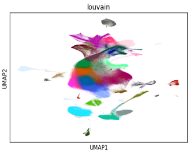
Figure 4: A sample visualization of the 1.3M mouse brain cells, reduced to 2 dimensions with UMAP from cuML and clustered with Louvain from cuGraph
Conclusion
At the rate in which our computational tools are advancing, we can assume it won’t be long before the data processing volumes catch up, especially for single-cell analysis workloads, forcing the need to scale ever higher. In the meantime, there are still opportunities to decrease the iteration times of the exploratory data analysis process even further by distributing the clustering and visualization steps over multiple GPUs. Faster iteration means better models, reduced time to insight, and more informed results. Except for T-SNE, all of the clustering and visualization steps of the multi-GPU workflow notebook can already be distributed over Dask workers on GPUs with RAPIDS cuML and cuGraph.
Understanding speed limit signs may seem like a straightforward task, but it can quickly become more complex in situations in which different restrictions apply to different lanes (for example, a highway exit) or when driving in a new country.
I am trying to implement simulated annealing using tensorflow_probability but I don’t understand how to update the transition kernel between steps correctly. I think I somehow have to use bijectors but I don’t really understand how. Can somehow explain it to me or link a working example?
Hello everyone! I’m having an issue when using TensorFlow under Jupyter (Anaconda).
When I try to create a Bidirectional layer, I always get this issue:
“Cannot convert a symbolic Tensor (bidirectional/forward_lstm/strided_slice:0) to a NumPy array. This error may indicate that you’re trying to pass a Tensor to a NumPy call, which is not supported”
It doesn’t matter the type of bidirectional layer, I always get this issue.
There are a number of factors businesses should consider to ensure an optimized edge computing strategy and deployment.
The growth of edge computing has been a hot topic in many industries. The value of smart infrastructure can mean improvements to overall operational efficiency, safety, and even the bottom line. However, not all workloads need to be, or even should be, deployed at the edge.
Enterprises use a combination of edge computing and cloud computing when developing and deploying AI applications. AI training typically takes place in the cloud or at data centers. When customers evaluate where to deploy AI applications for inferencing they consider aspects such as latency, bandwidth, and security requirements.
Edge computing is tailored for real-time, always-on solutions that have low latency requirements. Always-on solutions are sensors or other pieces of infrastructure that are constantly working or monitoring their environments. Examples of “always-on” solutions include networked video cameras for loss prevention, medical imaging in ERs for surgery support, or assembly line inspection in factories. Many customers have already embraced edge computing for AI applications. Read about how they are creating smarter, safer spaces.
As customers evaluate their AI strategy and where edge computing makes sense for their business, there are a number of factors they must consider to ensure an optimized deployment. These considerations include latency, scalability, remote management, security, and resiliency.
Lower Latency
Most are familiar with the idea of bringing compute to the data, not the other way around. This has a number of advantages. One of the most important is latency. Instead of losing time sending data back to the data center or the cloud, businesses process data in real time and derive intelligent insights instantly.
For example, retailers deploying AI loss prevention solutions cannot wait seconds or longer for a response to come back from their system. They need instant alerts for an abnormal behavior so that it can be flagged and dealt with immediately. Similarly, AI solutions designed for warehouses that detect when a worker is in the wrong place or not wearing the appropriate safety equipment needs an instantaneous response.
Scalability
Creating smart spaces often means that companies are looking to run AI at tens to thousands of locations. A major challenge to this scale is limited cloud bandwidth for moving and processing information. Bandwidth cap often leads to higher costs and smaller infrastructure. With edge computing solutions, data collection, and processing happens on the local network, bandwidth is tied to the local area network (LAN) and has a much broader range of scalability.
Remote Management
When scaling to hundreds of remote locations, one of the key considerations organizations must address is how to manage all edge systems. While some companies today have tried to employ skilled employees or contractors to handle provisioning and maintenance of edge locations, most quickly realize they need to centralize the management in order to scale. Edge management solutions make it easy for IT to provision edge systems, deploy AI software, and manage the ongoing updates needed.
Security
The security model for edge computing is almost entirely turned on its head compared to traditional security policies in the data center. While organizations can generally maintain physical security of their data center systems, edge systems are almost always freely accessible to many more people. This requires both physical hardware security processes to be put in place as well as software security solutions that can protect both the data and application security on these edge devices.
Resilience
Edge systems are generally managed with little or no skilled IT professionals on hand to assist in the event of a crash. Thus, edge management requires resilient infrastructure that can remediate issues on its own, as well as secure remote access when human intervention is required. Migrating applications when a system fails and restarting those applications automatically are core features of many cloud-native management solutions, making ongoing management of edge computing environments seamless.
There are numerous benefits driving customers to move their compute systems nearer to their data sources in remote locations. Customers need to consider how edge computing is different from data center or cloud computing they have traditionally relied on, and invest in new ways of provisioning, securing, and managing these environments.
Hey, I’m new to tensorflow although I’ve played around with image classification using python before,
I was wondering if it’s possible to input mp4 videos which also have related json objects which show hashtags, titles, usernames and likes etc for that video to train tensorflow with? I have a lot of these videos saved already (5,000+) along with their corresponding json and I wanted to try to train a neural net to see if it would pick similar videos that I would when inputting an mp4 and it’s json. Greatly appreciate any answers on whether this is possible and would work and pointing me in the right direction!
Hi everybody! It’s my first post here and I’m a beginner with TF too.
I’m trying to implement deep q-learning on the Connect 4 game. Reading some examples on the internet, I’ve understood that using the decorator tf.function can speed up a lot the training, but it has no other effect than performance.
Actually, I have noticed a different behavior in my function:
@tf.function # do I need it? def _train_step(self, boards_batch, scores_batch): with tf.GradientTape() as tape: batch_predictions = self.model(boards_batch, training=True) loss_on_batch = self.loss_object(scores_batch, batch_predictions) gradients = tape.gradient(loss_on_batch, self.model.trainable_variables) self.optimizer.apply_gradients(zip( gradients, self.model.trainable_variables )) self.loss(loss_on_batch)
In particular, if I train without tf.function the agent is not learning anything and it performs as the Random agent. Instead, if I use tf.function the agent easily beats the random agent after only 1000 episodes.
Do you have any idea why is this happening? Do I have misunderstood something about tf.function?
If I try to remove tf.function from TF example notebooks nothing changes a part from the performance, as I expect from my understanding of tf.function.

 From award-winning research demos to photorealistic graphics created with NVIDIA RTX and Omniverse, see how NVIDIA is breaking boundaries in AI, graphics, and virtual collaboration.
  Sign up for webinars with NVIDIA experts and Metropolis partners on Sept. 22, featuring developer SDKs, GPUs, go-to-market opportunities, and more.
  Learn how the use of RAPIDS to accelerate the analysis of single-cell RNA-sequence on a single NVIDIA V100 GPU shows a massive performance increase.
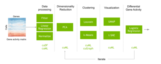
 There are a number of factors businesses should consider to ensure an optimized edge computing strategy and deployment.