SoftBank is a global technology player that aspires to drive the Information Revolution. The company operates in broadband, fixed-line telecommunications, ecommerce, information technology, finance, media, and marketing. To improve their users’ communication experience, and overcome the 5G capacity and coverage issues, SoftBank has used NVIDIA Maxine GPU-accelerated SDKs with state-of-the-art AI features to build virtual … Continued
SoftBank is a global technology player that aspires to drive the Information Revolution. The company operates in broadband, fixed-line telecommunications, ecommerce, information technology, finance, media, and marketing. To improve their users’ communication experience, and overcome the 5G capacity and coverage issues, SoftBank has used NVIDIA Maxine GPU-accelerated SDKs with state-of-the-art AI features to build virtual collaboration and content creation applications.
In this post, you learn how SoftBank used the Maxine SuperResolution and hardware-accelerated encode-decode operations to reduce the amount of data that must be uplinked to the multi-access edge computing (MEC) servers. Besides solving the challenge of limited bandwidth, Maxine features such as noise removal and virtual background enabled SoftBank to deliver the best video conferencing solution for their users.
Benefits of using MEC
Edge computing enables providers to deploy their technology closer to users. Simply put, edge computing reduces bandwidth and latency budgets for mission-critical, high-throughput, low-latency applications. This is achieved using MEC network technology to move the computing from a remote cloud server to a node closer to the consumption source. Edge computing relies heavily on network technologies such as 4G, and more recently 5G, to provide connectivity.
5G features such as ultra-high-speed, ultra-low latency, and multiple simultaneous connections enable new use cases such as telemedicine and smart factories that were previously unfeasible with wireless connectivity. MEC is the key to realizing the support of low-latency, high-throughput use cases. MEC reduces response delays by processing as much as possible at the edge by deploying regional MEC servers and sending only the minimum necessary data to the cloud. MEC servers often use the GPU massively parallel computing power for processing large amounts of data at high speed.
Challenges with the 5G network
The current 5G networks operate in a configuration called non-standalone (NSA). This configuration combines a 4G LTE network and a 5G base station, where some 5G features (such as network slicing) are not available. 5G SA (standalone) configuration has both a 5G core and a base station. 5G SA end-to-end support for 5G speeds services, reduces costs, improves the quality of service, and is a better platform for deploying services.
When the 5G SA configuration is in the market, the full 5G network is complete. In other words, 5G evolves in two steps: 5G NSA and 5G SA. Capital investment is required for each step.
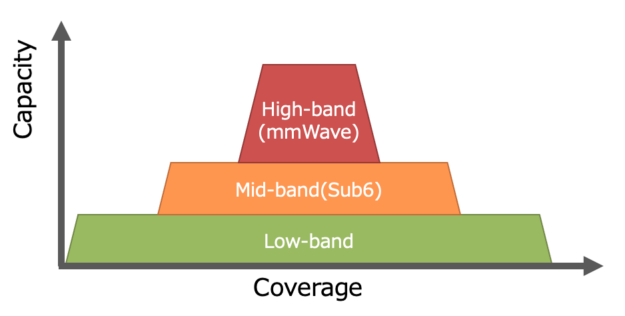
On the other hand, some telecom carriers, including SoftBank, have started using 4G LTE low-band frequency for 4G LTE and 5G NR. Theoretically, capacity and coverage are trade-offs in wireless communication. To ensure the high-quality, wide-area coverage for the 5G SA configuration, SoftBank uses MEC to effectively reduce service delays as much as possible.
In addition, there are some technical challenges. Mobile networks are generally designed to accommodate a higher downlink speed than uplink. This design philosophy works for general applications such as streaming videos on a smartphone, as most of the traffic is the downlink. However, some critical applications require a strong uplink connection. One of these is video conferencing, where the user needs considerable uplink bandwidth to stream high-resolution video and audio.
The current 5G uplink capacity is insufficient, and carrier aggregation and MIMO antennas are needed to provide more uplink allocation. As more and more devices connect to 5G, saving bandwidth, especially in the uplink, is a common challenge for all global telecom carriers.
Uplink bandwidth-intensive applications, such as video conferencing, can be served with the same quality of service at reduced uplink bandwidth (for example, 500 Kbps) as with ample bandwidth (100 Mbps). In those cases, it’s possible to connect many more devices and provide high-quality services at the same time.
Video conferencing solution on MEC with NVIDIA Maxine
NVIDIA Maxine is a GPU-accelerated SDK platform that enables developers of video conferencing services to build and deploy AI-powered features that use state-of-the-art models in the cloud. Maxine includes APIs using the latest innovations from NVIDIA research, such as artifact reduction, body pose estimation, super resolution, and noise removal. Maxine also uses other products, like NVIDIA Riva, to provide features like closed captioning and access to virtual assistants. These capabilities are fully accelerated on NVIDIA GPUs to run real-time video streaming applications in the cloud.
Maxine applications enable service providers to offer the same features to every user on any device, including computers, tablets, and phones. The key point is that all the processing happens on the cloud so that the application running on any device requires minimal resources. Applications built with Maxine are easily deployed as microservices and scale to hundreds of thousands of streams in a Kubernetes environment.
The idea is to offload the computationally intensive processing involved in video conferencing systems and reduce the amount of data that must be uplinked to the MEC servers. This is done through a combination of video effects like super resolution and hardware-accelerated encode-decode operations. Maxine also adds quality-of-life features like noise removal, virtual background, room echo cancelation, and more.
What does this mean for end users? Essentially, an end user with a low-bandwidth connection working onsite with a wide range of background noise can get connected with clean audio and a high-definition video. For instance, a plant manager at a noisy production floor in a remote location with a 180p stream connection can seem to be in a silent conference room with a 720p stream. The offloading of compute resources also translates to longer battery life and more free memory for the end user to multitask on resource-constrained devices like mobile phones and laptops.
The features mentioned earlier are housed in the following SDKs:
In addition, the NVIDIA Video Codec SDK provides hardware-accelerated encoding and decoding to aid the infrastructure around video conferencing.
How SoftBank used NVIDIA Maxine
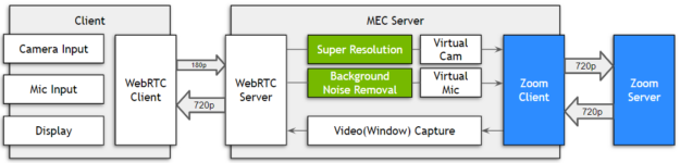
Typically, if you want to use a video conference solution on your mobile phone, you must first install a client application. In SoftBank’s case, the Zoom client is installed on the MEC server on the carrier network instead of the mobile phone. The video and microphone output of the mobile phone are inputs to the Zoom client on the MEC over the 5G network. MEC recognizes the smartphone’s microphone and camera as a virtual microphone and camera and uses them as input for the Zoom client.
Here are the hardware and software specifications used for the SoftBank proof of concept implementation:
- Hardware
- GPU: Quadro RTX6000 (driver version: 456.43)
- CPU: Intel Xeon Gold 6244
- Software
- Windows Server 2019
- NVIDIA Maxine Video Effects SDK (3/25/2021 – VFX – prerelease)
This work makes use of SoftBank’s MEC servers (Windows), a modified C++-based open source WebRTC client named “WebRTC Client Momo,” and an application that uses the Video Effect SDK and Audio Effect SDK API.
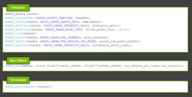
The NvAFX_RUN API (NVAFX_EFFECT_DENOISER) in AudioEffectSDK and NvVFX_RUN API (NVVFX_FX_SUPER_RES) in the Video Effect SDK are used to perform video super resolution and noise removal.
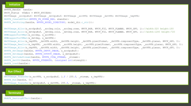
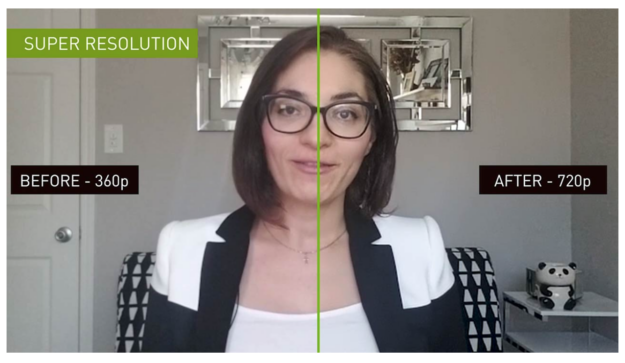
The video stream sent from the 5G user equipment using the WebRTC protocol is uploaded to the MEC at a low bit rate (in this verification, H.264 (CBR) 180p) to conserve uplink bandwidth. MEC receives degraded audio and video at low bit rates and improves quality using Maxine SDKs. For video, the MEC server uses the Maxine SuperResolution function to resize the video sent from the user equipment at 180p to 720p. SuperResolution reduces noise and restores high-frequency components, resulting in high-quality video.
Figure 8 shows the results of SuperResolution.

In Figure 8, the left side is the original data before applying SuperResolution, and the right side is the image upscaled. The blocky artifacts in the facial details are replaced with more pixels, leading to a high-quality image. You can replicate these results using the sample application provided with the Video Effects SDK. For a full demonstration, see this video. NEED VIDEO UPLOADED TO YOUTUBE OR DEVZONE
As with the Super Resolution result, the noise removal results are shown in the video.
The video shows the results of testing the Maxine noise removal feature in a scenario where the user is talking while typing on a keyboard. Here, keyboard sounds were selected as a sample, but noise removal was also useful in various situations throughout the development process of SoftBank’s PoC. SoftBank believes that noise removal makes noisy-environment meetings possible, such as outdoors or in a car.
You can replicate these results using the sample application provided with the Audio Effects SDK.
Improve the quality of your video stream
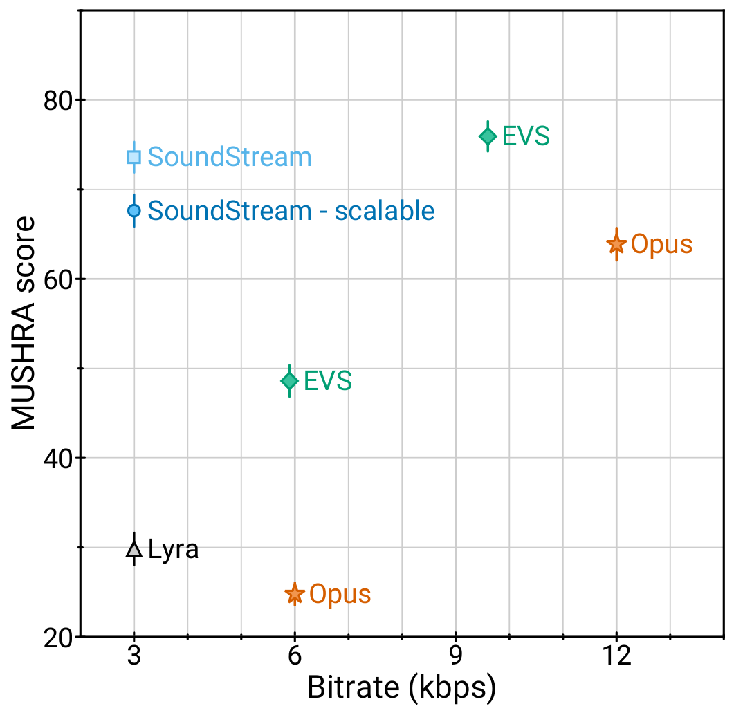
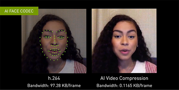
By deploying Maxine on their MEC servers, in addition to low latency, SoftBank now provides a high-quality video and audio experience to all end users. The improved end-user experience is achieved with high savings on the uplink bandwidth since no additional hardware or user equipment is needed. To improve the video quality further, SoftBank plans to use Maxine AI Face Codec.
For more information, see the GPU Virtualization for 5G and MEC Coexistence GTC session to learn more about SoftBank’s PoC or download Maxine SDKs to see how Maxine can improve your application. Contact us with any questions.


 With NVIDIA DriveWorks SDK, autonomous vehicles can bring their understanding of the world to a new dimension. The SDK enables autonomous vehicle developers to easily process three-dimensional lidar data and apply it to specific tasks, such as perception or localization. You can learn how to implement this critical toolkit in our expert-led webinar, Point Cloud …

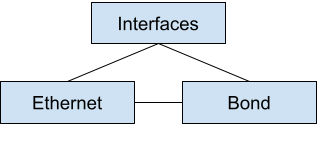
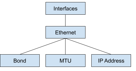
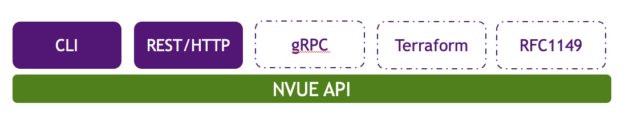
 Cumulus Linux 4.4 introduces a new CLI, NVUE, that is more than just a CLI. NVUE provides a complete object model for Linux, unlocking incredible operational potential.