
|
Hello everybody. I’m asking for help because I can’t find the math attribute. Some advice? I would like to use this optimizer : tfg.math.optimizer.levenberg_marquardt submitted by /u/Filippo9559 |
Tensorflow Graphics


|
Hello everybody. I’m asking for help because I can’t find the math attribute. Some advice? I would like to use this optimizer : tfg.math.optimizer.levenberg_marquardt submitted by /u/Filippo9559 |
A key challenge in natural language processing (NLP) is building conversational agents that can understand and reason about different language phenomena that are unique to realistic speech. For example, because people do not always premeditate exactly what they are going to say, a natural conversation often includes interruptions to speech, called disfluencies. Such disfluencies can be simple (like interjections, repetitions, restarts, or corrections), which simply break the continuity of a sentence, or more complex semantic disfluencies, in which the underlying meaning of a phrase changes. In addition, understanding a conversation also often requires knowledge of temporal relationships, like whether an event precedes or follows another. However, conversational agents built on today’s NLP models often struggle when confronted with temporal relationships or with disfluencies, and progress on improving their performance has been slow. This is due, in part, to a lack of datasets that involve such interesting conversational and speech phenomena.
To stir interest in this direction within the research community, we are excited to introduce TimeDial, for temporal commonsense reasoning in dialog, and Disfl-QA, which focuses on contextual disfluencies. TimeDial presents a new multiple choice span filling task targeted for temporal understanding, with an annotated test set of over ~1.1k dialogs. Disfl-QA is the first dataset containing contextual disfluencies in an information seeking setting, namely question answering over Wikipedia passages, with ~12k human annotated disfluent questions. These benchmark datasets are the first of their kind and show a significant gap between human performance and current state of the art NLP models.
TimeDial
While people can effortlessly reason about everyday temporal concepts, such as duration, frequency, or relative ordering of events in a dialog, such tasks can be challenging for conversational agents. For example, current NLP models often make a poor selection when tasked with filling in a blank (as shown below) that assumes a basic level of world knowledge for reasoning, or that requires understanding explicit and implicit inter-dependencies between temporal concepts across conversational turns.
It is easy for a person to judge that “half past one” and “quarter to two” are more plausible options to fill in the blank than “half past three” and “half past nine”. However, performing such temporal reasoning in the context of a dialog is not trivial for NLP models, as it requires appealing to world knowledge (i.e., knowing that the participants are not yet late for the meeting) and understanding the temporal relationship between events (“half past one” is before “three o’clock”, while “half past three” is after it). Indeed, current state-of-the-art models like T5 and BERT end up picking the wrong answers — “half past three” (T5) and “half past nine” (BERT).
The TimeDial benchmark dataset (derived from the DailyDialog multi-turn dialog corpus) measures models’ temporal commonsense reasoning abilities within a dialog context. Each of the ~1.5k dialogs in the dataset is presented in a multiple choice setup, in which one temporal span is masked out and the model is asked to find all correct answers from a list of four options to fill in the blank.
In our experiments we found that while people can easily answer these multiple choice questions (at 97.8% accuracy), state-of-the-art pre-trained language models still struggle on this challenge set. We experiment across three different modeling paradigms: (i) classification over the provided 4 options using BERT, (ii) mask filling for the masked span in the dialog using BERT-MLM, (iii) generative methods using T5. We observe that all the models struggle on this challenge set, with the best variant only scoring 73%.
| Model | 2-best Accuracy | |
| Human | 97.8% | |
| BERT – Classification | 50.0% | |
| BERT – Mask Filling | 68.5% | |
| T5 – Generation | 73.0% |
Qualitative error analyses show that the pre-trained language models often rely on shallow, spurious features (particularly text matching), instead of truly doing reasoning over the context. It is likely that building NLP models capable of performing the kind of temporal commonsense reasoning needed for TimeDial requires rethinking how temporal objects are represented within general text representations.
Disfl-QA
As disfluency is inherently a speech phenomenon, it is most commonly found in text output from speech recognition systems. Understanding such disfluent text is key to building conversational agents that understand human speech. Unfortunately, research in the NLP and speech community has been impeded by the lack of curated datasets containing such disfluencies, and the datasets that are available, like Switchboard, are limited in scale and complexity. As a result, it’s difficult to stress test NLP models in the presence of disfluencies.
| Disfluency | Example | |
| Interjection | “When is, uh, Easter this year?” | |
| Repetition | “When is Eas … Easter this year?” | |
| Correction | “When is Lent, I mean Easter, this year?” | |
| Restart | “How much, no wait, when is Easter this year?” |
| Different kinds of disfluencies. The reparandum (words intended to be corrected or ignored; in red), interregnum (optional discourse cues; in grey) and repair (the corrected words; in blue). |
Disfl-QA is the first dataset containing contextual disfluencies in an information seeking setting, namely question answering over Wikipedia passages from SQuAD. Disfl-QA is a targeted dataset for disfluencies, in which all questions (~12k) contain disfluencies, making for a much larger disfluent test set than prior datasets. Over 90% of the disfluencies in Disfl-QA are corrections or restarts, making it a much more difficult test set for disfluency correction. In addition, compared to earlier disfluency datasets, it contains a wider variety of semantic distractors, i.e., distractors that carry semantic meaning as opposed to simpler speech disfluencies.
| Passage: …The Normans (Norman: Nourmands; French: Normands; Latin: Normanni) were the people who in the 10th and 11th centuries gave their name to Normandy, a region in France. They were descended from Norse (“Norman” comes from “Norseman”) raiders and pirates from Denmark, Iceland and Norway who, under their leader Rollo, … |
| Q1: | In what country is Normandy located? | France ✓ | |
| DQ1: | In what country is Norse found no wait Normandy not Norse? | Denmark X | |
| Q2: | When were the Normans in Normandy? | 10th and 11th centuries ✓ | |
| DQ2: | From which countries no tell me when were the Normans in Normandy? | Denmark, Iceland and Norway X |
| A passage and questions (Qi) from SQuAD dataset, along with their disfluent versions (DQi), consisting of semantic distractors (like “Norse” and “from which countries”) and predictions from a T5 model. |
Here, the first question (Q1) is seeking an answer about the location of Normandy. In the disfluent version (DQ1) Norse is mentioned before the question is corrected. The presence of this correctional disfluency confuses the QA model, which tends to rely on shallow textual cues from the question for making predictions.
Disfl-QA also includes newer phenomena, such as coreference (expression referring to the same entity) between the reparandum and the repair.
| SQuAD | Disfl-QA | |
| Who does BSkyB have an operating license from? | Who removed [BSkyB’s] operating license, no scratch that, who do [they] have [their] operating license from? |
Experiments show that the performance of existing state-of-the-art language model–based question answering systems degrades significantly when tested on Disfl-QA and heuristic disfluencies (presented in the paper) in a zero-shot setting.
| Dataset | F1 | |
| SQuAD | 89.59 | |
| Heuristics | 65.27 (-24.32) | |
| Disfl-QA | 61.64 (-27.95) |
We show that data augmentation methods partially recover the loss in performance and also demonstrate the efficacy of using human-annotated training data for fine-tuning. We argue that researchers need large-scale disfluency datasets in order for NLP models to be robust to disfluencies.
Conclusion
Understanding language phenomena that are unique to human speech, like disfluencies and temporal reasoning, among others, is a key ingredient for enabling more natural human–machine communication in the near future. With TimeDial and Disfl-QA, we aim to fill a major research gap by providing these datasets as testbeds for NLP models, in order to evaluate their robustness to ubiquitous phenomena across different tasks. It is our hope that the broader NLP community will devise generalized few-shot or zero-shot approaches to effectively handle these phenomena, without requiring task-specific human-annotated training datasets, constructed specifically for these challenges.
Acknowledgments
The TimeDial work has been a team effort involving Lianhui Qi, Luheng He, Yenjin Choi, Manaal Faruqui and the authors. The Disfl-QA work has been a collaboration involving Jiacheng Xu, Diyi Yang, Manaal Faruqui.
 Machine Learning (ML) is increasingly used to make decisions across many domains like healthcare, education, and financial services. Since ML models are being used in situations that have a real impact on people, it is critical to understand what features are being considered for the decisions to eliminate or minimize the impact of biases. Model … Continued
Machine Learning (ML) is increasingly used to make decisions across many domains like healthcare, education, and financial services. Since ML models are being used in situations that have a real impact on people, it is critical to understand what features are being considered for the decisions to eliminate or minimize the impact of biases.
Model Interpretability aids developers and other stakeholders to understand model characteristics and the underlying reasons for the decisions, thus making the process more transparent. Being able to interpret models can help data scientists explain the reasons for decisions made by their models, adding value and trust to the model. In this post, we discuss:
There are six main reasons that justify the need for model interoperability in machine learning:
Understanding fairness issues in the model: An interpretable model can explain the reasons for choosing the outcome. In social contexts, these explanations will inevitably reveal inherent biases towards underrepresented groups. The first step to overcoming these biases is to see how they manifest.
A more precise understanding of the objectives: The need for explanations also arises from our gaps in understanding the problem fully. Explanations are one of the ways to ensure that the effects of the gaps are visible to us. It helps in understanding whether the models’ predictions are matching the stakeholders’ or experts’ objectives.
Creating Robust Models: Interpretable models can help us understand why there’s some variance in the predictions, which can help make them more robust and eliminate extreme and unintended changes in forecasts; and why the errors were made. Increasing robustness can also help build trust in the model as it doesn’t produce dramatically different results.
Model interpretability can also help debug models, explain outcomes to stakeholders, and enable auditing to meet regulatory compliances.
It is important to note that there are instances where interpretability might be less important. For example, there might be cases where adding interpretable models can aid adversaries to cheat the systems.
Now that we understand what interpretability is and why we need it, let’s look at one way of implementing it that has become very popular recently.
There are different methods that aim at improving model interpretability; one such model-agnostic method is SHAPley Values. It’s a method derived from coalitional game theory to provide a way to distribute the “payout” across the features fairly. In the case of Machine Learning models, the payout is the predictions/outcome of the models. It works by computing the Shapley Values for the whole dataset and combining them.
cuML, the Machine Learning library in RAPIDS that supports single and multi-GPU Machine Learning algorithms, provides GPU-accelerated Model Explainability through Kernel Explainer and Permutation Explainer. Kernel SHAP is the most versatile and commonly used black box explainer of SHAP. It uses weighted linear regression to estimate the SHAP values, making it a computationally efficient method to approximate the values.
The cuML implementation of Kernel SHAP provides acceleration to fast GPU models, like those in cuML. They can also be used with CPU-based models, where speedups can still be achieved but they might be limited due to data transfers and the speed of models themselves.
In the next section, we will discuss how to use RAPIDS Kernel SHAP on Azure.
InterpretML is an open-source package that incorporates state-of-the-art machine learning interpretability techniques under one roof. While the main interpretability techniques and glass box explainable models are covered in the Interpret package of this offering, Interpret-Community extends the Interpret repository and incorporates further community developed and experimental interpretability techniques and functionalities that are designed to enable interpretability for real-world scenarios.
We can extend this to explain models on Microsoft Azure, which is discussed in more detail later. Interpret-community provides various techniques for interpreting models, including:
To make GPU-accelerated SHAP easily accessible to end-users, we integrated the cuML’s GPU KernelExplainer to the interpret-community package. Users who have access to VMs with GPUs on Azure (NVIDIA Pascal or better) can install RAPIDS (>=0.20) and enable the GPU explainer by setting the use_gpu flag to True.
from interpret.ext.blackbox import TabularExplainer

# "features" and "classes" fields are optional
explainer = TabularExplainer(model,
                          x_train,
                          features=breast_cancer_data.feature_names,
                          classes=classes,
use_gpu=True)
The newly added GPUKernelExplainer also uses cuML K-Means to replicate the behavior of shap.kmeans. KMeans reduces the size of background data to be processed by the explainers. It summarizes the dataset passed with K mean samples weighted by the number of data points. Replacing sklearn K-Means with cuML allows us to leverage the speed-ups of GPU even during preprocessing of the data before SHAP.
Based on our experiments, we found that cuML models, when used with cuML KernelExplainer, produce the most optimal results for speeds noticing up to 270x speed-ups in some cases. We also saw the best speed-ups for models with optimized and fast predict calls, as seen with the optimized sklearn.svm.LinearSVR and cuml.svm.SVR(kernel=’linear’).
Azure Machine Learning provides a way to get explanations for regular and automated ML training through the azureml-interpret SDK package. It enables the user to achieve model interpretability on real-world datasets at scale during training and inference[2]. We can also use interactive visualizations to further explore overall and individual model predictions and understand our model and dataset further. Azure-interpret uses the techniques in the interpret-community package, which means it now supports RAPIDS SHAP. We’ll walk through an example notebook demonstrating Model Interpretability using cuML’s SHAP on Azure.
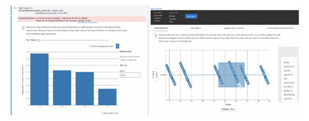
We benchmarked the CPU and GPU implementation on a single explain_global call in Azure. The explain_global function returns the aggregate feature importance values as opposed to instance-level feature importance values while using explain_local. We are comparing cuml.svm.SVR(kernel=’rbf’) vs sklearn.svm.SVR(kernel=’rbf’) on synthetic data with shape (10000, 40).
As we can observe from Table 1, when we use the GPU VM (Standard_NC6S_v3), there’s a 420x speed-up on 2000 rows of explanation as opposed to a CPU VM with 16 cores (Standard_DS5_v2). We did notice that using a 64-core CPU VM(Standard_D64S_v3) over a 16-core CPU VM yielded a faster CPU runtime (by the order of around 1.3x). This faster CPU run was still much slower than the GPU run and more expensive. GPU run was 380x faster with a cost of $0.52 in comparison to a $23 for the 64 core CPU VM. We ran the experiments in the US East region in Azure.
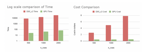

From our experiments, using cuML’s KernelExplainer proves to be more cost and time-efficient on Azure. The speed-ups are better as the number of rows increases. Not only does GPU SHAP explain more data but it also saves more money and time. This can hugely impact businesses that are time-sensitive.
A simple example of how you can use cuML’s SHAP for explanations on Azure. This can be extended to larger examples with more interesting models and datasets. The libraries discussed in this post are constantly updated, if you’re interested in adding or requesting new features check out the following resources:
 Ray Tracing Games II is now available to download for free via Apress and Amazon. This Open Access book is a must-have for anyone interested in real-time rendering. Ray tracing is the holy grail of gaming graphics, simulating the physical behavior of light to bring real-time, cinematic-quality rendering to even the most visually intense games.
Ray Tracing Games II is now available to download for free via Apress.
This Open Access book is a must-have for anyone interested in real-time rendering. Ray tracing is the holy grail of gaming graphics, simulating the physical behavior of light to bring real-time, cinematic-quality rendering to even the most visually intense games. Ray tracing is also a fundamental algorithm used for architecture applications, visualization, sound simulation, deep learning, and more.
To win a limited edition print copy of Ray Tracing Gems II, enter the giveaway contest here: https://developer.nvidia.com/ray-tracing-gems-ii
A message from the editors:
In 2018, real-time ray tracing arrived in consumer GPU hardware and swiftly established itself as a key component of how images would be generated moving forward. Now, three years later, the second iteration of this hardware is available, mainstream game consoles support ray tracing, and cross-platform API standards have been established to drive even wider adoption. Developers and researchers have been busy inventing (and reinventing) algorithms to take advantage of the new possibilities created by these advancements. The “gems” of knowledge discovered during this process are what you will find in Ray Tracing Gems II.
Before diving into the treasure trove, we want to make sure you know the following:
Open access content allows you to freely copy and redistribute any chapter, or the whole book, as long as you give appropriate credit and you are not using it for commercial purposes. The specific license is the Creative Commons Attribution 4.0 International License (CC-BY-NC-ND). We put this in place so that authors, and everyone else, can disseminate the information in this volume as quickly, widely, and equitably as possible.
Writing an anthology style book, such as this, is an act of collective faith. Faith that the authors, editors, publisher, and schedules all converge to produce a worthwhile result for readers. Under normal circumstances this is a difficult task, but the past year and a half has been anything but “normal”. This book’s call for participation was posted in late November 2019, just as the COVID-19 virus began to emerge in Asia. In the 18 months since, a once-in-a-century pandemic has surged. Its impact has touched every person on Earth – and it is not yet over. The virus has taken lives, battered livelihoods, and broken the way of life as we knew it. We postponed this book with the quiet conviction that the coronavirus would be overcome. As time passed, the development of vaccines made breakneck progress, remote work in quarantine became a new staple of life, and authors began to write about computer graphics again. As a result, this book was written entirely during quarantine. We sincerely thank the authors for their passion and dedication – and faith – all of which made this book possible under extraordinary circumstances.
– Adam Marrs, Peter Shirley, and Ingo Wald
Sustainability isn’t just a choice for consumers to make. It’s an opportunity for companies to lead. AI startup Heartdub seams together fashion and technology to let designers and creators display physical fabrics and garments virtually — and help clothing companies achieve zero-waste manufacturing. The company’s software digitizes textiles and then simulates how clothes look on Read article >
The post Zero Waste with Taste: Startup Uses AI to Drive Sustainable Fashion appeared first on The Official NVIDIA Blog.
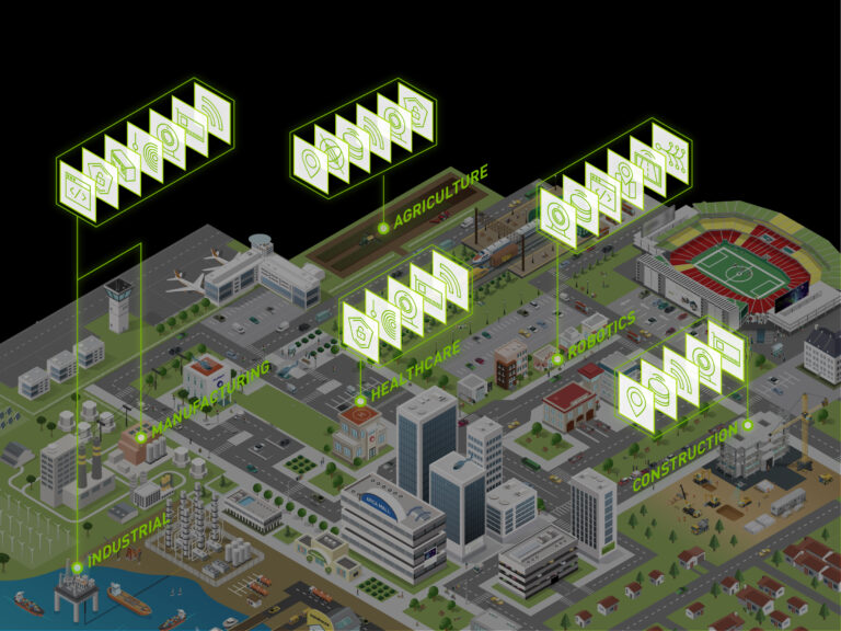 A new generation of AI applications at the edge is driving incredible operational efficiency and safety gains across a broad range of spaces. Read how the power of AI and edge computing is critical to building smarter and safer spaces.

In an increasingly complex world, the need to automate and improve operational efficiency and safety in our physical spaces has never been greater. Whether it is streamlining the retail experience, tackling traffic congestion in our growing cities, or improving productivity in our factories—the power of AI and edge computing is critical.
Video cameras are one of the most important IoT sensors. With approximately 1 billion cameras deployed worldwide, they generate a wealth of data that, when combined with AI-enabled perception and reasoning, is key to transforming ordinary areas into smart spaces.
As the number of IoT sensors grows, more data is getting generated in remote edge locations. Sending data from sensors at the edge to data centers is extremely costly. However, data movement is critical for the successful operation of AI applications, which means that these applications are susceptible to high costs and latency when processing through the cloud. Sending the data to data centers is not ideal in contexts where every second counts, such as managing real-time traffic or addressing medical emergencies.
This leads us to edge computing, a distributed computing model that allows computing to take place near the sensor where data is being collected and analyzed.
Edge computing is the technology that powers edge AI, an architecture that processes the sensor data with deep learning algorithms close to the sensors generating the data. Edge AI enables any device or computer to process data and make decisions in real-time with minimal latency. Hence, edge computing is essential for real-time applications that require low latency to enable quick responses. Examples include spotting obstacles on rail lines, inspecting defects on fast moving assembly lines, or detecting patient falls in hospitals.
By bringing AI processing tasks closer to the source, edge computing overcomes issues that can occur with cloud computing, like high latency and compromised security. Some advantages of edge computing are:
Use Cases of Edge Computing for Smart Cities
Cities, school campuses, and shopping malls are several of many places that have started to use AI at the edge to transform themselves into smart spaces. From traffic management to city planning, these entities are using AI to make their spaces more efficient, accessible, and safe.
The following examples illustrate how edge computing has been used to transform operations and improve safety around the world.
To reduce traffic congestion
Nota developed a real-time traffic control solution that uses edge computing and computer vision to identify traffic volume, analyze congestion, and optimize traffic signal controls at intersections. Nota’s solutions are used by cities to improve traffic flow, saving them traffic congestion-related costs and minimizing the amount of time drivers spend in traffic. [Read more]
To assess and avoid operational hazards in cities
Viisights helps manage operations within Israel’s cities. Viisights’ edge computing application assists city officials in identifying and managing events in densely populated areas. Its real-time detection of behavior helps officials predict how quickly an event is growing and determine if there is reason for alarm or a need to take action. [Read more]
To revolutionize the retail industry
Many retail stores and distribution centers use edge computing and computer vision to bring real-time insights to retailers, enabling them to protect their assets and streamline distribution system processes. The technology can help retailers grow their top line with efficiencies that can improve retailers’ net profit margins. [Read more]
To save lives at beaches
Sightbit developed an image detection application that helps spot dangers at beaches. Speed is very critical in these life or death situations which is why processing is done at the edge. The system detects potential dangers such as rip currents, or hazardous ocean conditions allowing authorities to enact life-saving procedures. [Read more]
To improve airline and airport operation efficiency
Airports around the world are partnering with ASSAIA to use edge computing to improve turnaround times and reduce delays. ASSAIA’s AI-enabled video analytics application produces insights that help airlines and airports make better and quicker decisions around capacity, sustainability, and safety. [Read more]
A new generation of AI applications at the edge is driving incredible operational efficiency and safety gains across a broad range of spaces. Download this free e-book to learn how edge computing is helping build smarter and safer spaces around the world.
Modern workloads such as AI and machine learning are putting tremendous pressure on traditional IT infrastructure. Enterprises that want to stay ahead of these changes can now register to participate in an early access of Project Monterey, an initiative to dramatically improve the performance, manageability and security of their environments. VMware, Dell Technologies and NVIDIA Read article >
The post Soar into the Hybrid-Cloud: Project Monterey Early Access Program Now Available to Enterprises appeared first on The Official NVIDIA Blog.
 Azure recently announced support for NVIDIA’s T4 Tensor Core Graphics Processing Units (GPUs) which are optimized for deploying machine learning inferencing or analytical workloads in a cost-effective manner. With Apache Spark™ deployments tuned for NVIDIA GPUs, plus pre-installed libraries, Azure Synapse Analytics offers a simple way to leverage GPUs to power a variety of data … Continued
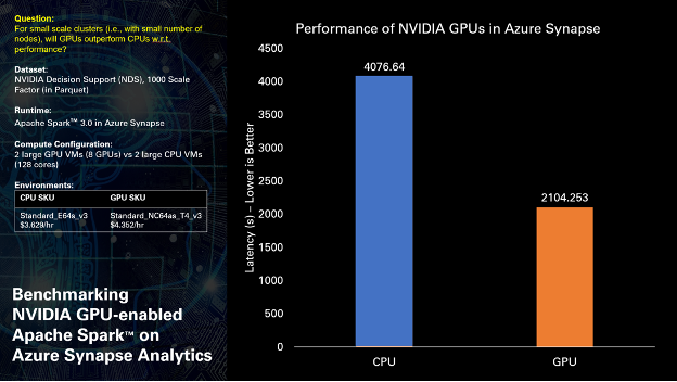
Azure recently announced support for NVIDIA’s T4 Tensor Core Graphics Processing Units (GPUs) which are optimized for deploying machine learning inferencing or analytical workloads in a cost-effective manner. With Apache Spark deployments tuned for NVIDIA GPUs, plus pre-installed libraries, Azure Synapse Analytics offers a simple way to leverage GPUs to power a variety of data processing and machine learning tasks. With built-in support for RAPIDS acceleration, the Azure Synapse version of GPU-accelerated Spark offers at least 2x performance gain on standard analytical benchmarks compared to running on CPUs, all without any code changes.
Currently, this GPU acceleration feature in Azure Synapse is available for private preview by request.
NVIDIA GPUs offer extraordinarily high compute performance, bringing parallel processing to multi-core servers to accelerate demanding workloads. A CPU consists of a few cores optimized for sequential serial processing, whereas. On the other hand, a GPU has a massively parallel architecture consisting of thousands of smaller and more efficient cores designed to handle multiple tasks simultaneously. Considering that data scientists spend up to 80% of their time on data pre-processing, GPUs are a critical tool to accelerate data processing pipelines compared to relying on pipelines containing CPUs alone.
One of the most efficient and familiar ways to build these pipelines is using Apache Spark . The benefits of NVIDIA GPU acceleration in Apache Spark
 include:
NVIDIA and Azure Synapse have teamed up to bring GPU acceleration to data scientists and data engineers. This integration will give customers the freedom to use NVIDIA GPUs for Apache Spark applications with no-code changes and with an experience identical to a CPU cluster. In addition, this collaboration will continue to add support for the latest NVIDIA GPUs and networking products and provide continuous enhancements for big data customers who are looking to improve productivity and save costs with a single pipeline for data engineering, data preparation, and machine learning.
To learn more about this project, check out our presentation at NVIDIA’s GTC 2021 Conference.
 3.0 GPU Acceleration in Azure Synapse
While Apache Spark provides GPU support out-of-box, configuring and managing all the required hardware and installing all the low-level libraries can take significant effort. When you try GPU-enabled Apache Spark
 pools in Azure Synapse, you will immediately notice a surprisingly simple user experience:
Behind the scenes heavy lifting: To efficiently use GPUs, libraries are used to perform communication with the graphics card on the host machine. Installing and configuring these libraries takes time and effort. Azure Synapse takes care of pre-installing these libraries and setting up all the complex networking between compute nodes through integration with GPU Apache Spark pools. Within just a few minutes, you can stop worrying about setup and focus on solving business problems.
Optimized Spark configuration: By collaborating between NVIDIA and Azure Synapse, we have come up with optimal configurations for your GPU-enabled Apache Spark pools. Thus, your workloads run most optimally saving you both time and operational costs.
Packed with Data Prep and ML Libraries: The GPU-enabled Apache Spark pools in Azure Synapse come built-in with two popular libraries with support for more on the way:
 enables GPU-accelerated SQL, DataFrame operations, and Spark shuffles. Since there are no code changes required to leverage these accelerations, you can also accelerate your data pipelines that rely on Linux Foundation’s Delta Lake or Microsoft’s Hyperspace indexing (both of which are available on Synapse out-of-box).
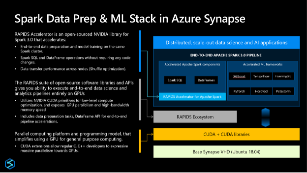
When running NVIDIA Decision Support (NDS) test queries, derived from industry-known benchmarks, over 1 TB of Parquet data our early results indicate that GPUs can deliver nearly 2x acceleration in overall query performance, without any code changes.
Hi
I’m not sure what’s going on with my classification model, as it predicts objects as floats instead of classes. Is it something to do with the loss function or activation functions at the end of the network?
The barebones code can be found here:
submitted by /u/dahkneela
[visit reddit] [comments]
Say I would like to quickly remove an object from my dataset. Can I drop all samples with the specific id (say id=7), and then remove the definition of the label with id=7 from the label_map file (making it skip from 6 straight to 8)?
Or is it expected that the ids are contiguous, so that I have to shift all labels (8 and up) down by one after removing 7?
submitted by /u/Meriipu
[visit reddit] [comments]