Categories
Misc

Maximizing Network Performance for Storage with NVIDIA Spectrum Ethernet

As data generation continues to increase, linear performance scaling has become an absolute requirement for scale-out storage. Storage networks are like car…

As data generation continues to increase, linear performance scaling has become an absolute requirement for scale-out storage. Storage networks are like car roadway systems: if the road is not built for speed, the potential speed of a car does not matter. Even a Ferrari is slow on an unpaved dirt road full of obstacles.

Scale-out storage performance can be hindered by the Ethernet fabric that connects the storage nodes. NVIDIA accelerated Ethernet can remove performance bottlenecks, enabling maximum storage performance for applications in general, and AI/ML in particular.

Scale-out storage requires a strong network

Every second, 54,000 pictures are taken worldwide. By the time you read this, that number will be even higher. No matter what your business is, chances are you have massive amounts of data that must be stored and analyzed, with the amount growing every day. 

The old scale-up approach of using ever-larger storage filers has been replaced with a scale-out approach to deliver storage that scales linearly in both capacity and performance.

With scale-out storage, or distributed storage, several smaller nodes are configured and connected to act as one logical unit. A single file or object can be spread across many nodes. 

As more scale is needed, additional storage nodes are easily added to increase both storage capacity and performance. This applies to both a traditional enterprise storage vendor solution, or a software-defined solution, with the software and hardware sourced independently. 

Distributed storage enables flexible scaling and cost efficiency, but requires a high-performance network to connect the storage nodes. Many data center switches are ill-suited to the unique traffic characteristics of storage, and in fact can cripple the performance of scale-out storage solutions.  

How storage traffic is different from traditional traffic

For many use cases, network traffic is consistent and homogeneous, and traditional Ethernet suffices. However, traffic generated by storage devices may cause the issues detailed below.

Network stress 

Current storage solutions benefit from faster SSDs and storage interfaces, such as NVMe and PCIe Gen 4 (soon PCIe Gen 5), that are designed to provide higher performance. 

Congestion 

When the storage fabric is saturated, network congestion becomes inevitable, just like roadway congestion when too much traffic is on the highway. Network congestion is particularly problematic for scale-out storage because each storage node is expected to offer fast data delivery. But when congestion occurs, many data center switches have a fairness problem, where some nodes will be slowed much more than others. A single file or object is usually spread across many nodes, so anything that slows a single node effectively slows the whole cluster.

Bursty traffic

Most storage workloads are bursty, generating intense data transfers and repeatedly requiring large amounts of bandwidth for short periods. When that happens, the network switch must use its buffer to absorb the burst until the transient burst is over, thus preventing packet loss. Otherwise, that packet loss will require data retransmissions, significantly deteriorating application performance.

Storage jumbo frames 

Traditional data center network traffic uses a maximum packet size (MTU) of 1.5 KB. Scale-out storage nodes perform better when they can use 9 KB “jumbo frames,” which increase throughput while reducing ‌CPU processing overhead. Many data center switches built with commodity switch ASICs perform poorly or unpredictably with jumbo frames.

Low latency 

One of the ways storage IOPs have improved is through the orders-of-magnitude latency reduction for the read/write operations in flash-based media. ‌However, those costly performance improvements can be lost when the network introduces high latency—especially due to excessive buffering.

Both training and inference require adequate amounts of data with high-speed access, to make sure that GPU processors are fed quickly enough to keep them fully engaged. During training, WRITE operations are performed by all nodes to improve model accuracy. This results in a burst, making it imperative for switches to handle congestion effectively. Finally, lower storage latency enables GPUs to handle compute tasks more efficiently.

Why ASICs are suboptimal for storage traffic 

Most data center switches are built using commodity switch ASICs that were cost-optimized for traditional data traffic patterns and packet sizes. To keep costs low while achieving their bandwidth targets, Ethernet switch chip vendors compromised fairness by using a split buffer architecture.

Every switch has a buffer to absorb traffic bursts and prevent packet loss when congestion occurs. The common approach is to have a buffer that is shared across many ports. However, not all shared buffers are the same—there are different buffer architectures.

Commodity switches do not have a fully shared buffer—they use either an ingress-shared buffer, or an egress-shared buffer. 

With an ingress-shared buffer, there is a static mapping between a group of incoming ports and a specific memory slice. These ports can use only the memory in that assigned slice and not the whole buffer, not even if the rest of the buffer is available and no one is using it. 

With an egress-shared buffer, the mapping is between a group of outgoing ports and a specific buffer memory slice. Again, each group of egress ports can only use its assigned buffer slice, not the whole buffer.

With these two architectures, flows that stay within the same memory slice do not behave like flows that travel between memory slices. If many flows use ports with the same buffer, those ports will experience higher latency and lower throughput, while traffic using other slices of the buffer will enjoy higher performance. 

The storage performance depends on which ports the storage traffic (and other traffic) is using and how busy are the buffer slices for those ports. This is why switches that use split buffers often experience issues related to fairness, predictability, and microburst absorption.

Why deep-buffer switches are suboptimized for storage 

Deep-buffer switches usually refer to a switch that offers much more buffering (GBs rather than MBs). Deep-buffer switches are often promoted for use as routers, because they can absorb and hold large traffic bursts if there is a mismatch in network speeds or an incast situation. 

But in most data center applications, including scale-out storage, the deep-buffer switches negatively impact performance for the following reasons:

Job completion time 

With parallel file systems, the storage node with the slowest response dictates the time required to fetch a file. Unlike commodity switch ASICs that have a sliced on-chip buffer, deep-buffer switches have both on-chip and off-chip buffers, and they all are sliced, not fully shared, buffers. 

Think of how many ways flows can go before they leave the switch. They can stay within one on-chip memory slice (fastest), travel between on-chip memory slices (slower), or travel between on-chip and off-chip memory slices (very slow). 

All these flows will behave differently, and hence will cause fairness and predictability issues for storage traffic. Because these issues slow down one or more nodes, they adversely impact job completion time and slow down the whole distributed storage cluster.

Latency

The larger the switch buffer, the longer the queue each packet must go through and the greater the latency. The tested average port-to-port latency of a deep-buffer switch is more than 500 microseconds. Compared to a fully shared buffer switch from the same generation, NVIDIA Spectrum 1 latency is just 0.3 microseconds. It requires nanoseconds rather than microseconds to switch/route a packet. 

Deep-buffer latency is 1,000x higher. You may be wondering, is this just happening when congestion occurs? No. Under congestion, deep-buffer latencies will be much higher; in fact, up to 20 milliseconds, or 50,000x higher. While 500 microseconds of latency might be okay for a router between data centers, within a data center it spells death to flash storage performance.

Power and cost 

Deep-buffer switches need hundreds of watts of power to operate even when idling, making their ongoing operational cost higher. The initial purchase cost of deep-buffer switches is also much higher. This might be justified if performance was better, but real-world testing has proven just the opposite. 

Choosing an inappropriate network switch will severely slow down your storage workloads, making your expensive fast storage act like cheaper and slower storage. 

With NVIDIA Spectrum, both CapEx and OpEx can be reduced. Watts can also be used for other purposes within a rack.  

NVIDIA Spectrum switches are optimized for storage

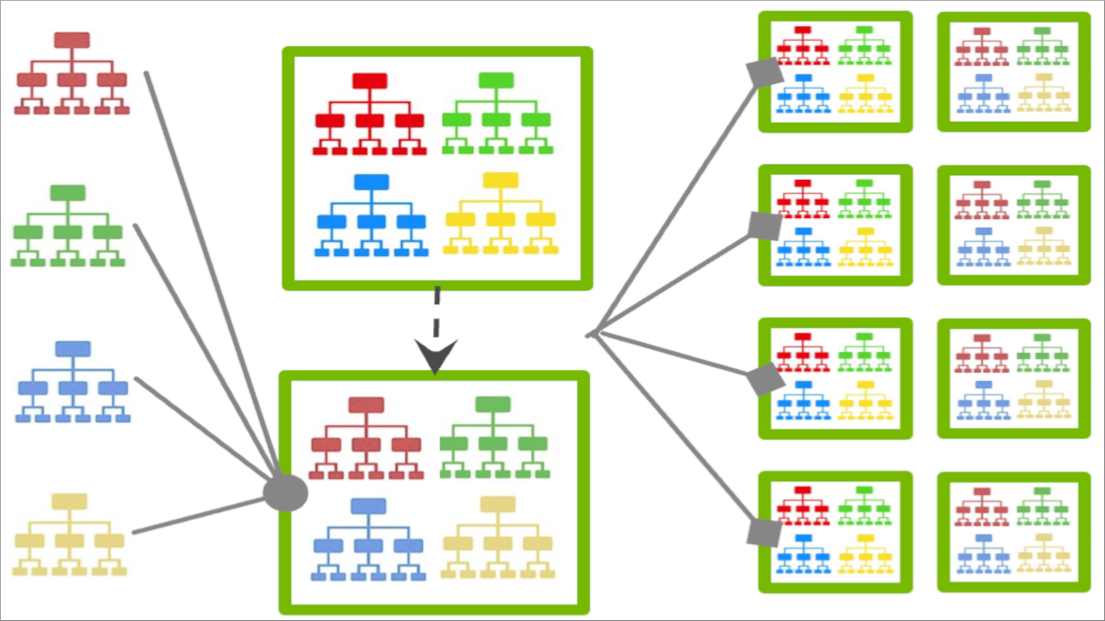
With commodity switch ASICs, flows are either staying at the same memory slice or traveling between memory slices. 

With NVIDIA Spectrum switches, all flows behave the same due to the fully shared buffer. The value of this architecture is maximum burst absorption capacity as well as optimal fair and predictable performance. All traffic flows through a switch receive the same treatment and generally enjoy the same good performance, regardless of which ingress and egress ports they use.

Benchmarking the deep-buffer switch and NVIDIA Spectrum

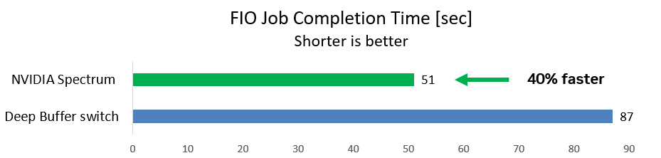
The first case uses a common storage benchmarking FIO tool for WRITE operations from two initiators to one target while background traffic is running. This is a typical storage scenario. 

The team measured the time required for the FIO job to complete (shorter is better). With the deep-buffer switch, the FIO job took 87 seconds. With the NVIDIA Spectrum switch, the job ran 40% faster and completed after just 51 seconds.

Bar graph comparing NVIDIA Spectrum and deep-buffer switch showing that NVIDIA Spectrum is 40% faster at job completion time.
Figure 1. Storage write operations are 40% faster with the NVIDIA Spectrum switch compared to a deep-buffer switch

Deep-buffer switches greatly increase latency, which slows down your storage and reduces your application performance. But how high can the latency go?

For the second case, the team took the deep-buffer switch and tested how latency is impacted under different congestion use cases. The maximum buffer occupancy is only around 10% of the whole buffer size.

Two line graphs comparing real and projected latency compared to buffer size and buffer occupancy.
Figure 2. Real and projected latency compared to buffer size and buffer occupancy

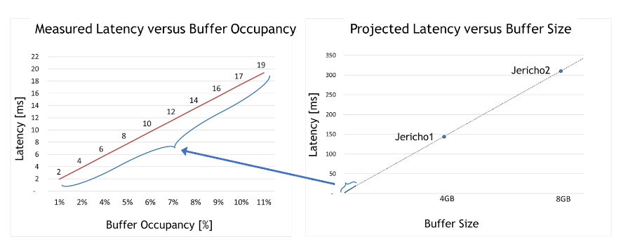
Two meaningful insights can be derived from the graph on the left of Figure 2. First, deep-buffer switch latency is 50,000x higher than Spectrum switches (2–19 milliseconds compared to only 300 nanoseconds for Spectrum). 

Second, linear dependency is apparent between buffer occupancy and latency. In other words, testing proved that the larger the occupied buffer, the greater the latency.

With that understanding, the graph on the right of Figure 2 projects the maximum latency per deep-buffer ASIC (such as Jericho 1, Jericho 2, or Ramon). These very high latency numbers are incompatible with data center applications in general and fast storage solutions in particular.

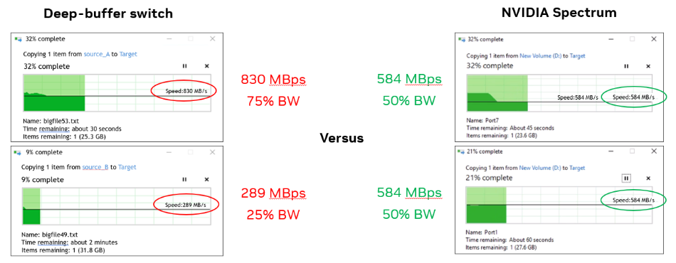
For the third case, the team used two Windows machines and simultaneously copied a file from each to the same target storage.

With the deep-buffer switch, one Windows machine had three times the bandwidth of the other (830 MBps compared to 290 MBps). With Spectrum switch, each machine had 584 MBps (50% as expected).

Real-world testing showed that deep-buffer switches do not have a positive impact on data center applications, such as absorbing packets and preventing drops.

Deep-buffer switches may be needed for long haul or WAN connections; however, they are suboptimal for data center applications and will have negative effects, particularly when the workload is scaled beyond just two nodes, as in this use case. 

Two stacked graphs comparing the deep-buffer switch and NVIDIA Spectrum, where the bandwidth performance is better with the NVIDIA Spectrum and noted in green.
Figure 3. The deep-buffer switch provides unfair bandwidth per node (left) while the NVIDIA Spectrum switch provides equal bandwidth (right)

These three use cases demonstrate proof points for why deep-buffer switches adversely impact AI/ML and storage workloads, while Spectrum switches provide maximized performance.

Summary

NVIDIA Spectrum Ethernet switches are built for AI/ML and storage workloads, and perform better than switches with split buffers or deep buffers. They handle congestion better, prevent packet loss, and outperform with jumbo frames (preferred for storage). NVIDIA Spectrum Ethernet switches provide overall good application performance with consistently low network latency.

Learn more about NVIDIA Spectrum Ethernet switches. Dive deeper into networking storage in the NVIDIA Developer Forums

Categories
Offsites

Preference learning with automated feedback for cache eviction

Caching is a ubiquitous idea in computer science that significantly improves the performance of storage and retrieval systems by storing a subset of popular items closer to the client based on request patterns. An important algorithmic piece of cache management is the decision policy used for dynamically updating the set of items being stored, which has been extensively optimized over several decades, resulting in several efficient and robust heuristics. While applying machine learning to cache policies has shown promising results in recent years (e.g., LRB, LHD, storage applications), it remains a challenge to outperform robust heuristics in a way that can generalize reliably beyond benchmarks to production settings, while maintaining competitive compute and memory overheads.

In “HALP: Heuristic Aided Learned Preference Eviction Policy for YouTube Content Delivery Network”, presented at NSDI 2023, we introduce a scalable state-of-the-art cache eviction framework that is based on learned rewards and uses preference learning with automated feedback. The Heuristic Aided Learned Preference (HALP) framework is a meta-algorithm that uses randomization to merge a lightweight heuristic baseline eviction rule with a learned reward model. The reward model is a lightweight neural network that is continuously trained with ongoing automated feedback on preference comparisons designed to mimic the offline oracle. We discuss how HALP has improved infrastructure efficiency and user video playback latency for YouTube’s content delivery network.

Learned preferences for cache eviction decisions

The HALP framework computes cache eviction decisions based on two components: (1) a neural reward model trained with automated feedback via preference learning, and (2) a meta-algorithm that combines a learned reward model with a fast heuristic. As the cache observes incoming requests, HALP continuously trains a small neural network that predicts a scalar reward for each item by formulating this as a preference learning method via pairwise preference feedback. This aspect of HALP is similar to reinforcement learning from human feedback (RLHF) systems, but with two important distinctions:

  • Feedback is automated and leverages well-known results about the structure of offline optimal cache eviction policies.
  • The model is learned continuously using a transient buffer of training examples constructed from the automated feedback process.

The eviction decisions rely on a filtering mechanism with two steps. First, a small subset of candidates is selected using a heuristic that is efficient, but suboptimal in terms of performance. Then, a re-ranking step optimizes from within the baseline candidates via the sparing use of a neural network scoring function to “boost” the quality of the final decision.

As a production ready cache policy implementation, HALP not only makes eviction decisions, but also subsumes the end-to-end process of sampling pairwise preference queries used to efficiently construct relevant feedback and update the model to power eviction decisions.

A neural reward model

HALP uses a light-weight two-layer multilayer perceptron (MLP) as its reward model to selectively score individual items in the cache. The features are constructed and managed as a metadata-only “ghost cache” (similar to classical policies like ARC). After any given lookup request, in addition to regular cache operations, HALP conducts the book-keeping (e.g., tracking and updating feature metadata in a capacity-constrained key-value store) needed to update the dynamic internal representation. This includes: (1) externally tagged features provided by the user as input, along with a cache lookup request, and (2) internally constructed dynamic features (e.g., time since last access, average time between accesses) constructed from lookup times observed on each item.

HALP learns its reward model fully online starting from a random weight initialization. This might seem like a bad idea, especially if the decisions are made exclusively for optimizing the reward model. However, the eviction decisions rely on both the learned reward model and a suboptimal but simple and robust heuristic like LRU. This allows for optimal performance when the reward model has fully generalized, while remaining robust to a temporarily uninformative reward model that is yet to generalize, or in the process of catching up to a changing environment.

Another advantage of online training is specialization. Each cache server runs in a potentially different environment (e.g., geographic location), which influences local network conditions and what content is locally popular, among other things. Online training automatically captures this information while reducing the burden of generalization, as opposed to a single offline training solution.

Scoring samples from a randomized priority queue

It can be impractical to optimize for the quality of eviction decisions with an exclusively learned objective for two reasons.

  1. Compute efficiency constraints: Inference with a learned network can be significantly more expensive than the computations performed in practical cache policies operating at scale. This limits not only the expressivity of the network and features, but also how often these are invoked during each eviction decision.
  2. Robustness for generalizing out-of-distribution: HALP is deployed in a setup that involves continual learning, where a quickly changing workload might generate request patterns that might be temporarily out-of-distribution with respect to previously seen data.

To address these issues, HALP first applies an inexpensive heuristic scoring rule that corresponds to an eviction priority to identify a small candidate sample. This process is based on efficient random sampling that approximates exact priority queues. The priority function for generating candidate samples is intended to be quick to compute using existing manually-tuned algorithms, e.g., LRU. However, this is configurable to approximate other cache replacement heuristics by editing a simple cost function. Unlike prior work, where the randomization was used to tradeoff approximation for efficiency, HALP also relies on the inherent randomization in the sampled candidates across time steps for providing the necessary exploratory diversity in the sampled candidates for both training and inference.

The final evicted item is chosen from among the supplied candidates, equivalent to the best-of-n reranked sample, corresponding to maximizing the predicted preference score according to the neural reward model. The same pool of candidates used for eviction decisions is also used to construct the pairwise preference queries for automated feedback, which helps minimize the training and inference skew between samples.

An overview of the two-stage process invoked for each eviction decision.

Online preference learning with automated feedback

The reward model is learned using online feedback, which is based on automatically assigned preference labels that indicate, wherever feasible, the ranked preference ordering for the time taken to receive future re-accesses, starting from a given snapshot in time among each queried sample of items. This is similar to the oracle optimal policy, which, at any given time, evicts an item with the farthest future access from all the items in the cache.

Generation of the automated feedback for learning the reward model.

To make this feedback process informative, HALP constructs pairwise preference queries that are most likely to be relevant for eviction decisions. In sync with the usual cache operations, HALP issues a small number of pairwise preference queries while making each eviction decision, and appends them to a set of pending comparisons. The labels for these pending comparisons can only be resolved at a random future time. To operate online, HALP also performs some additional book-keeping after each lookup request to process any pending comparisons that can be labeled incrementally after the current request. HALP indexes the pending comparison buffer with each element involved in the comparison, and recycles the memory consumed by stale comparisons (neither of which may ever get a re-access) to ensure that the memory overhead associated with feedback generation remains bounded over time.

Overview of all main components in HALP.

Results: Impact on the YouTube CDN

Through empirical analysis, we show that HALP compares favorably to state-of-the-art cache policies on public benchmark traces in terms of cache miss rates. However, while public benchmarks are a useful tool, they are rarely sufficient to capture all the usage patterns across the world over time, not to mention the diverse hardware configurations that we have already deployed.

Until recently, YouTube servers used an optimized LRU-variant for memory cache eviction. HALP increases YouTube’s memory egress/ingress — the ratio of the total bandwidth egress served by the CDN to that consumed for retrieval (ingress) due to cache misses — by roughly 12% and memory hit rate by 6%. This reduces latency for users, since memory reads are faster than disk reads, and also improves egressing capacity for disk-bounded machines by shielding the disks from traffic.

The figure below shows a visually compelling reduction in the byte miss ratio in the days following HALP’s final rollout on the YouTube CDN, which is now serving significantly more content from within the cache with lower latency to the end user, and without having to resort to more expensive retrieval that increases the operating costs.

Aggregate worldwide YouTube byte miss ratio before and after rollout (vertical dashed line).

An aggregated performance improvement could still hide important regressions. In addition to measuring overall impact, we also conduct an analysis in the paper to understand its impact on different racks using a machine level analysis, and find it to be overwhelmingly positive.

Conclusion

We introduced a scalable state-of-the-art cache eviction framework that is based on learned rewards and uses preference learning with automated feedback. Because of its design choices, HALP can be deployed in a manner similar to any other cache policy without the operational overhead of having to separately manage the labeled examples, training procedure and the model versions as additional offline pipelines common to most machine learning systems. Therefore, it incurs only a small extra overhead compared to other classical algorithms, but has the added benefit of being able to take advantage of additional features to make its eviction decisions and continuously adapt to changing access patterns.

This is the first large-scale deployment of a learned cache policy to a widely used and heavily trafficked CDN, and has significantly improved the CDN infrastructure efficiency while also delivering a better quality of experience to users.

Acknowledgements

Ramki Gummadi is now part of Google DeepMind. We would like to thank John Guilyard for help with the illustrations and Richard Schooler for feedback on this post.

Categories
Misc

Deep Learning Digs Deep: AI Unveils New Large-Scale Images in Peruvian Desert

Researchers at Yamagata University in Japan have harnessed AI to uncover four previously unseen geoglyphs — images on the ground, some as wide as 1,200 feet, made using the land’s elements — in Nazca, a seven-hour drive south of Lima, Peru. The geoglyphs — a humanoid, a pair of legs, a fish and a bird Read article >

Categories
Misc

Speech AI Spotlight: Visualizing Spoken Language and Sounds on AR Glasses

Image of glasses with computer screen reflected.Audio can include a wide range of sounds, from human speech to non-speech sounds like barking dogs and sirens. When designing accessible applications for people…Image of glasses with computer screen reflected.

Audio can include a wide range of sounds, from human speech to non-speech sounds like barking dogs and sirens. When designing accessible applications for people with hearing difficulties, the application should be able to recognize sounds and understand speech.

Such technology would help deaf or hard-of-hearing individuals with visualizing speech, like human conversations and non-speech sounds. Combining speech and sound AI together, you can overlay the visualizations onto AR glasses, making it possible for users to see and interpret sounds that they wouldn’t be able to hear otherwise. 

According to the World Health Organization, about 1.5B people (nearly 20% of the global population) live with hearing loss. This number could rise to 2.5B by 2050.

Cochl, an NVIDIA partner based in San Jose, is a deep-tech startup that uses sound AI technology to understand any type of audio. They are also a member of the NVIDIA Inception Program, which helps startups build their solutions faster by providing access to cutting-edge technology and NVIDIA experts.

The platform can recognize 37 environmental sounds, and the company went one step further by adding cutting-edge speech-to-text technology. This gives a truly complete understanding of the world of sound.

AR glasses to visualize any sound

AR glasses have the potential to greatly improve the lives of people with hearing loss as an accessible tool to visualize sounds. This technology can help enhance their communication abilities and make it easier for them to navigate and participate in the world around them.

Video 1. Cochl.Sense and NVIDIA Riva working on Microsoft HoloLens 2!

In this scenario, automatic speech recognition (ASR) is used to enable the glasses to recognize and understand human speech. This technology can be integrated into the glasses in several ways:

  • Using a microphone to capture the speech of a person talking to a deaf or hard-of-hearing individual and then using ASR algorithms to interpret and transcribe the speech into text. This text can then be displayed on the glasses, enabling the deaf or hard-of-hearing person to read and understand the speech.
  • ASR can also be used to enable the glasses to respond to voice commands so that users can control the glasses with their voice.
  • They are also able to display all conversations on the screen, such as transcribing voice directions from maps while you drive and any other sounds like horns or sirens from emergency vehicles and wind noise.

The technology behind the solution

Cochl used NVIDIA Riva to power its ASR capabilities within its software stack. Riva is a GPU-accelerated, fully customizable SDK for developing speech AI applications. By using Riva, the platform has been able to expand its capabilities to understand a wide range of sounds, including non-speech sounds.

“We’ve tested lots of speech recognition services, but only Riva provided exceptionally high and stable real-time performance. So now we can make our sound AI system be closer to human auditory perception,” said Yoonchang Han, co-founder and CEO at Cochl.

“As we have observed, AR glasses are most likely to be used in open spaces with noisy environments. NVIDIA Riva has helped us transcribe speech accurately even in noisy environments and has given us a seamless experience to integrate into our Cochl.Sense platform.”

Future of assistive technology

Creating a generalized AI system that perceives sounds like humans is a huge challenge. To make AR glasses more accessible, lighter wearable technology is required.

However, at this point, they are still an ideal medium for translating sounds and speech to visual information. By integrating machine listening functionality, AR glasses can bring safer, more convenient, and more enjoyable daily life to deaf or hard-of-hearing people all around the world.

Cochl is also exploring more use cases for speech AI, such as offering closed captioning for any videos on AR glasses and visualizing multi-speaker transcriptions. To provide the best experience for individuals with hearing difficulties, they are exploring ways to analyze and visualize music to help them understand the genre and emotion of the music at a minimum.

They are excited to experiment with more NVIDIA solutions including Riva, NVIDIA NeMo, and NVIDIA TensorRT.

Get started with speech AI today

Interested in adding speech AI to your VR applications? Browse these resources to get started:

Categories
Misc

Model Parallelism and Conversational AI Workshops

person typing at computer.Join these upcoming workshops to learn how to train large neural networks, or build a conversational AI pipeline.person typing at computer.

Join these upcoming workshops to learn how to train large neural networks, or build a conversational AI pipeline.

Categories
Offsites

SoundStorm: Efficient parallel audio generation

The recent progress in generative AI unlocked the possibility of creating new content in several different domains, including text, vision and audio. These models often rely on the fact that raw data is first converted to a compressed format as a sequence of tokens. In the case of audio, neural audio codecs (e.g., SoundStream or EnCodec) can efficiently compress waveforms to a compact representation, which can be inverted to reconstruct an approximation of the original audio signal. Such a representation consists of a sequence of discrete audio tokens, capturing the local properties of sounds (e.g., phonemes) and their temporal structure (e.g., prosody). By representing audio as a sequence of discrete tokens, audio generation can be performed with Transformer-based sequence-to-sequence models — this has unlocked rapid progress in speech continuation (e.g., with AudioLM), text-to-speech (e.g., with SPEAR-TTS), and general audio and music generation (e.g., AudioGen and MusicLM). Many generative audio models, including AudioLM, rely on auto-regressive decoding, which produces tokens one by one. While this method achieves high acoustic quality, inference (i.e., calculating an output) can be slow, especially when decoding long sequences.

To address this issue, in “SoundStorm: Efficient Parallel Audio Generation”, we propose a new method for efficient and high-quality audio generation. SoundStorm addresses the problem of generating long audio token sequences by relying on two novel elements: 1) an architecture adapted to the specific nature of audio tokens as produced by the SoundStream neural codec, and 2) a decoding scheme inspired by MaskGIT, a recently proposed method for image generation, which is tailored to operate on audio tokens. Compared to the autoregressive decoding approach of AudioLM, SoundStorm is able to generate tokens in parallel, thus decreasing the inference time by 100x for long sequences, and produces audio of the same quality and with higher consistency in voice and acoustic conditions. Moreover, we show that SoundStorm, coupled with the text-to-semantic modeling stage of SPEAR-TTS, can synthesize high-quality, natural dialogues, allowing one to control the spoken content (via transcripts), speaker voices (via short voice prompts) and speaker turns (via transcript annotations), as demonstrated by the examples below:

Input: Text (transcript used to drive the audio generation in bold)        Something really funny happened to me this morning. | Oh wow, what? | Well, uh I woke up as usual. | Uhhuh | Went downstairs to have uh breakfast. | Yeah | Started eating. Then uh 10 minutes later I realized it was the middle of the night. | Oh no way, that’s so funny!        I didn’t sleep well last night. | Oh, no. What happened? | I don’t know. I I just couldn’t seem to uh to fall asleep somehow, I kept tossing and turning all night. | That’s too bad. Maybe you should uh try going to bed earlier tonight or uh maybe you could try reading a book. | Yeah, thanks for the suggestions, I hope you’re right. | No problem. I I hope you get a good night’s sleep
         
Input: Audio prompt       


Output: Audio prompt + generated audio       


SoundStorm design

In our previous work on AudioLM, we showed that audio generation can be decomposed into two steps: 1) semantic modeling, which generates semantic tokens from either previous semantic tokens or a conditioning signal (e.g., a transcript as in SPEAR-TTS, or a text prompt as in MusicLM), and 2) acoustic modeling, which generates acoustic tokens from semantic tokens. With SoundStorm we specifically address this second, acoustic modeling step, replacing slower autoregressive decoding with faster parallel decoding.

SoundStorm relies on a bidirectional attention-based Conformer, a model architecture that combines a Transformer with convolutions to capture both local and global structure of a sequence of tokens. Specifically, the model is trained to predict audio tokens produced by SoundStream given a sequence of semantic tokens generated by AudioLM as input. When doing this, it is important to take into account the fact that, at each time step t, SoundStream uses up to Q tokens to represent the audio using a method known as residual vector quantization (RVQ), as illustrated below on the right. The key intuition is that the quality of the reconstructed audio progressively increases as the number of generated tokens at each step goes from 1 to Q.

At inference time, given the semantic tokens as input conditioning signal, SoundStorm starts with all audio tokens masked out, and fills in the masked tokens over multiple iterations, starting from the coarse tokens at RVQ level q = 1 and proceeding level-by-level with finer tokens until reaching level q = Q.

There are two crucial aspects of SoundStorm that enable fast generation: 1) tokens are predicted in parallel during a single iteration within a RVQ level and, 2) the model architecture is designed in such a way that the complexity is only mildly affected by the number of levels Q. To support this inference scheme, during training a carefully designed masking scheme is used to mimic the iterative process used at inference.

SoundStorm model architecture. T denotes the number of time steps and Q the number of RVQ levels used by SoundStream. The semantic tokens used as conditioning are time-aligned with the SoundStream frames.

Measuring SoundStorm performance

We demonstrate that SoundStorm matches the quality of AudioLM’s acoustic generator, replacing both AudioLM’s stage two (coarse acoustic model) and stage three (fine acoustic model). Furthermore, SoundStorm produces audio 100x faster than AudioLM’s hierarchical autoregressive acoustic generator (top half below) with matching quality and improved consistency in terms of speaker identity and acoustic conditions (bottom half below).

Runtimes of SoundStream decoding, SoundStorm and different stages of AudioLM on a TPU-v4.
Acoustic consistency between the prompt and the generated audio. The shaded area represents the inter-quartile range.

Safety and risk mitigation

We acknowledge that the audio samples produced by the model may be influenced by the unfair biases present in the training data, for instance in terms of represented accents and voice characteristics. In our generated samples, we demonstrate that we can reliably and responsibly control speaker characteristics via prompting, with the goal of avoiding unfair biases. A thorough analysis of any training data and its limitations is an area of future work in line with our responsible AI Principles.

In turn, the ability to mimic a voice can have numerous malicious applications, including bypassing biometric identification and using the model for the purpose of impersonation. Thus, it is crucial to put in place safeguards against potential misuse: to this end, we have verified that the audio generated by SoundStorm remains detectable by a dedicated classifier using the same classifier as described in our original AudioLM paper. Hence, as a component of a larger system, we believe that SoundStorm would be unlikely to introduce additional risks to those discussed in our earlier papers on AudioLM and SPEAR-TTS. At the same time, relaxing the memory and computational requirements of AudioLM would make research in the domain of audio generation more accessible to a wider community. In the future, we plan to explore other approaches for detecting synthesized speech, e.g., with the help of audio watermarking, so that any potential product usage of this technology strictly follows our responsible AI Principles.

Conclusion

We have introduced SoundStorm, a model that can efficiently synthesize high-quality audio from discrete conditioning tokens. When compared to the acoustic generator of AudioLM, SoundStorm is two orders of magnitude faster and achieves higher temporal consistency when generating long audio samples. By combining a text-to-semantic token model similar to SPEAR-TTS with SoundStorm, we can scale text-to-speech synthesis to longer contexts and generate natural dialogues with multiple speaker turns, controlling both the voices of the speakers and the generated content. SoundStorm is not limited to generating speech. For example, MusicLM uses SoundStorm to synthesize longer outputs efficiently (as seen at I/O).

Acknowledgments

The work described here was authored by Zalán Borsos, Matt Sharifi, Damien Vincent, Eugene Kharitonov, Neil Zeghidour and Marco Tagliasacchi. We are grateful for all discussions and feedback on this work that we received from our colleagues at Google.

Categories
Misc

Overview of Zero-Shot Multi-Speaker TTS Systems: Top Q&As

Title slide for Speech AI Summit session.The Speech AI Summit is an annual conference that brings together experts in the field of AI and speech technology to discuss the latest industry trends and…Title slide for Speech AI Summit session.

The Speech AI Summit is an annual conference that brings together experts in the field of AI and speech technology to discuss the latest industry trends and advancements. This post summarizes the top questions asked during Overview of Zero-Shot Multi-Speaker TTS System, a recorded talk from the 2022 summit featuring Coqui.ai.

Synthesizing a voice with seconds of audio

Text-to-speech (TTS) systems have significantly advanced in recent years with deep learning approaches. These advances have motivated research that aims to synthesize speech into the voice of a target speaker using just a few seconds of speech. This approach is called zero-shot multi-speaker TTS. The Coqui.ai session explored the timeline and state-of-the-art technology behind this approach.

Here are some key takeaways from the session:

  • YourTTS achieved state-of-the-art performance in English and showed the feasibility of performing zero-shot multi-speaker TTS in a target language by using a single-speaker dataset. This opened possibilities for the development of these systems in low-resource languages, such as indigenous languages. For more information, see YourTTS: Towards Zero-Shot Multi-Speaker TTS and Zero-Shot Voice Conversion for Everyone.
  • Advances in speaker verification systems can improve the performance of zero-shot multi-speaker TTS systems.
  • Zero-shot multi-speaker TTS can be used to generate new artificial voices. This is achieved by sampling a new speaker embedding. The new speaker embedding can be a completely random vector or interpolation between different speaker embeddings. For example, you could generate voices without copyrighting.

Top Q&As for zero-shot multi-speaker TTS systems

Can you create entirely brand new voices? Are there benefits to zero-shot to consider over one-minute fine-tuning? What are the hardware requirements to train a TTS model? Edresson Casanova dives into the top questions for developing zero-shot multi-speaker TTS systems.

How is text-to-speech quality measured?

Generally, the quality and naturalness of a TTS system are evaluated using the mean opinion score (MOS). With this metric, human evaluators listen to the audio and give a score on a scale between one and five, with one indicating bad quality and five indicating excellent quality.

In zero-shot multi-speaker TTS systems, you must also evaluate the similarity for new speakers by using a similarity MOS. In addition, a speaker encoder is used to measure speaker similarity. Compute the speaker encoder cosine similarity (SECS) where the speakers’ embeddings for two audio samples are extracted, and the cosine similarity between these embeddings is computed.

Researchers have recently published papers that explore the use of artificial neural networks to predict the MOS. At present, the generalization of these systems is not good enough, especially for new recording conditions, such as a different microphone or noise environment.

Can speech-to-text systems be used to measure text-to-speech system quality?

Speech-to-text (STT) systems can be used to check if the TTS model’s pronunciation is right, but it is not so much used in literature. Evaluation with an STT model covers only pronunciation and not the quality aspects of the speech itself.

What is the benefit of zero-shot compared to one-minute fine-tuning?

Zero-shot can work well, but not always. In some recordings, conditions and voices are too different from those seen in training. The zero-shot can fail and produce a voice not as similar to the target speaker’s voice. In this case, one-minute fine-tuning can be used. The YourTTS paper shows that the model can learn voices well, even for voices where the model has had a bad zero-shot.

How important is the architecture of the speaker encoder? Do you suggest training the speaker encoder separately or along with the spectrogram generator?

The speaker encoder is one of the most important components for the final quality of zero-shot multi-speaker TTS models. Without good speaker embeddings, the model can’t clone new voices. The speaker encoder used on the YourTTS model was pretrained separately on thousands of speakers, and it was kept frozen during the training.

Some papers—such as Attentron: Few-Shot Text-to-Speech Utilizing Attention-Based Variable-Length Embedding—show that training a speaker encoder-like module along with the TTS model could produce good results. In my experience, it depends on how many speakers you have in the training set. Without adequate speaker diversity, the model easily overfits and does not work well with speakers or recording conditions not seen in training.

Is it possible to interpolate speaker encoder representation to create an unseen voice as a mix of known voices?

It is possible. It is also able to generate new artificial voices through a random speaker embedding. Although the YourTTS colab demos do not cover it, the SC-GlowTTS colab demo shows an example of how to generate a completely new artificial voice.

Are models phoneme-based or character-based for training?

YourTTS is character-based. However, for example, Sc-GlowTTS is phoneme-based. On YourTTS, we decided to train it using characters instead of phonemes because the objective of this model is to be used in low-resource languages that normally do not have good phonemizers.

How much data center compute is required to train your leading text-to-speech model?

YourTTS used one NVIDIA V100 32-GB GPU with a batch size of 64. However, it is possible to train it with a smaller batch size using GPUs with less VRAM. I have never tried a GPU with less VRAM, but I know that some Coqui TTS contributors have already fine-tuned the YourTTS model using GPUs with 11 GB of VRAM.

When computing the speaker embeddings, does it help to exclude certain segments from embedding extraction like silence or unvoiced or plosive phonemes?

Although the speaker encoder should learn how to ignore the silences and focus just on speech, during the dataset preprocessing step, we removed beginning and end long silences to avoid problems during the model training. Then, we removed long silences. However, we do not remove unvoiced or plosive phonemes segments.

Can zero-shot text-to-speech be achieved for expressive speech?

It can be achieved. At Coqui.ai, we have already developed a model that can do zero-shot multi-speaker TTS and generates expressive speech in five different emotions. This model is available through Coqui Studio.

More resources

From fine-tuning a model to generating a custom voice, speech AI technology helps organizations tackle complex conversations globally. Check out the following resources to learn how your organization can integrate speech AI into core operations.

Categories
Misc

Applying Federated Learning to Traditional Machine Learning Methods

In the era of big data and distributed computing, traditional approaches to machine learning (ML) face a significant challenge: how to train models…

In the era of big data and distributed computing, traditional approaches to machine learning (ML) face a significant challenge: how to train models collaboratively when data is decentralized across multiple devices or silos. This is where federated learning comes into play, offering a promising solution that decouples model training from direct access to raw training data.

One of the key advantages of federated learning, which was initially designed to enable collaborative deep learning on decentralized data, is its communication efficiency. This same paradigm can be applied to traditional ML methods such as linear regression, SVM, k-means clustering, and tree-based methods like random forest and boosting.

Developing a federated-learning variant of traditional ML methods requires careful considerations that must be made at several levels:

  • Algorithm level: You must answer crucial questions such as what information clients should share with the server, how the server should aggregate the collected information, and what clients should do with the global aggregated model updates received from the server.
  • Implementation level: It’s essential to explore available APIs and harness them to create a federated pipeline that aligns with the algorithm formulation.

It’s worth noting that the line between federated and distributed machine learning can be less distinct for traditional methods compared to deep learning. For some algorithms and implementations, these terms can be equivalent.

Hierarchical diagram shows how federated tree-based XGBoost aggregates a collection of trees, then redistributes to clients for further training.
Figure 1. A high-level approach to federated tree-based XGBoost

In Figure 1, each client builds a unique boosted tree that is aggregated by the server as a collection of trees and then redistributed to clients for further training.

To get started with a specific example that shows this approach, consider the k-means clustering example. Here we followed the scheme defined in Mini-Batch K-Means clustering and formulated each round of federated learning as follows:

  • Local training: Starting from global centers, each client trains a local MiniBatchKMeans model with their own data.
  • Global aggregation: The server collects the cluster center, counts information from all clients, aggregates them by considering each client’s results as a mini-batch, and updates the global center and per-center counts.

For center initialization, at the first round, each client generates its initial centers with the k-means++ method. Then, the server collects all initial centers and performs one round of k-means to generate the initial global center.

From formulation to implementation

Applying a federated paradigm to traditional machine learning methods is easier said than done. The new NVIDIA whitepaper, Federated Traditional Machine Learning Algorithms, provides numerous detailed examples to show how to formulate and implement these algorithms.

Employing popular libraries like scikit-learn and XGBoost, we showcase how federated linear models, k-means clustering, non-linear SVM, random forest, and XGBoost can be adapted for collaborative learning.

In conclusion, federated machine learning offers a compelling approach to training models collaboratively on decentralized data. While communication costs may no longer be the principal constraint for traditional machine learning algorithms, careful formulation and implementation are still necessary to fully leverage the benefits of federated learning.

To get started with your own federated machine learning workflows, see the Federated Traditional Machine Learning Algorithms whitepaper and the NVIDIA FLARE GitHub repo.

Categories
Misc

Scientists Improve Delirium Detection Using AI and Rapid-Response EEGs

Detecting delirium isn’t easy, but it can have a big payoff: speeding essential care to patients, leading to quicker and surer recovery. Improved detection also reduces the need for long-term skilled care, enhancing the quality of life for patients while decreasing a major financial burden. In the U.S., caring for those suffering from delirium costs Read article >

Categories
Misc

A Golden Age: ‘Age of Empires III’ Joins GeForce NOW

Conquer the lands in Microsoft’s award-winning Age of Empires III: Definitive Edition. It leads 10 new games supported today on GeForce NOW. At Your Command Age of Empires III: Definitive Edition is a remaster of one of the most beloved real-time strategy franchises featuring improved visuals, enhanced gameplay, cross-platform multiplayer and more. Command mighty civilizations Read article >