In this output, the first (3, 3) is the spatial width and height of the filters/kernels applied in this conv layer. The third 3 refers to the number of input channels provided to this layer and 64 refers to the number of filters applied.
How can I access the 64 filters applied in this conv layer?
I am trying to train an Autoencoder using TensorFlow2.5 and Python3.8 as follows: Inception NetV3 was used to perform feature extraction using an image dataset containing 289229 images. The final output of Inception NetV3 is 2048-d vector. I pickled all of them in a Python3 list and load it along with the filenames:
# Read pickled Python3 list containing 2048-d extracted feature representation per image- features_list = pickle.load(open("DeepFashion_features_inceptionnetv3.pickle", "rb")) # Convert from Python3 list to numpy array- features_list_np = np.asarray(features_list) features_list_np.shape # (289229, 2048) del features_list # Read pickled Python3 list containing abolute path and filenames- filenames_list = pickle.load(open("DeepFashion_filenames_inceptionnetv3.pickle", "rb")) len(features_list), len(filenames_list) # (289229, 289229) # Note that the absolute path contains Google colab path- filenames_list[1] # '/content/img/1981_Graphic_Ringer_Tee/img_00000002.jpg' # Create 'tf.data.Dataset' using np array- batch_size = 32 features_list_dataset = tf.data.Dataset.from_tensor_slices(features_list_np).batch(batch_size) x = next(iter(features_list_dataset)) # 2021-06-28 13:10:00.229937: W tensorflow/core/kernels/data/model_dataset_op.cc:205] Optimization loop failed: Cancelled: Operation was cancelled x.shape # TensorShape([32, 2048])
My first question is why does it give the message “Optimization loop failed”? I am using Nvidia RTX 3080 with 16GB GPU. Note that since this is an autoencoder, there are no accompanying labels for the given data!
Is there any other better way of feeding this Python3 list as input to a TF2 neural network that I am missing?
I am checking for available GPU:
num_gpus = len(tf.config.list_physical_devices('GPU')) print(f"number of GPUs available = {num_gpus}") # number of GPUs available = 1
Second, I coded an autoencoder with the architecture:
I understand that you need to create the forward propagation, and let tensorflow deals with the backward propagation
my model goes like this
We start with initialization (HE method)
def initialize_HE(arr):
params={}
for i in range(1,len(arr)):
l=str(i)
params[‘W’+l] = tf.Variable(tf.random.normal((arr[i],arr[i-1])),name=’W’+l) * np.sqrt(2 / arr[i-1])
params[‘b’+l] = tf.Variable(tf.zeros((arr[i],1)),name=’b’+l)
return params
this will give me a dictionary of W1,W2,b1,b2 …etc
the forward goes like this
def forward(params,X,types):
L = len(types)
out = {}
out[‘A0’]=X
for i in range(1,L+1):
l = str(i)
l0 = str(i-1)
out[‘Z’+l] = params[‘W’+l] @ out[‘A’+l0] + params[‘b’+l]
if types[i-1] ==’relu’:
out[‘A’+l] = tf.nn.relu(out[‘Z’+l])
if types[i-1] == ‘sigmoid’:
out[‘A’+ l] = tf.nn.sigmoid(out[‘Z’+l])
return out[‘A’+ l]
This will give me the last layer output, let’s call it y_hat
so far I’m only replacing numpy variables with tensorflow’s
Learn how NVIDIA NGC and NVIDIA Clara (NVIDIA’s healthcare AI Platform) can help accelerate medical imaging workflows.
The NVIDIA NGC team is hosting a webinar with live Q&A to dive into our new Jupyter notebook available from the NGC catalog. Learn how to use these resources to kickstart your AI journey.
NVIDIA NGC Jupyter Notebook Day: Building a 3D Medical Imaging Segmentation Model Thursday, July 22 at 9:00 AM PT
Image segmentation deals with placing each pixel (or voxel in the case of 3D) of an image into specific classes that share common characteristics. In medical imaging, image segmentation can be used to help identify organs and anomalies, measure them, classify them, and even uncover diagnostic information by using data gathered from x-rays, magnetic resonance imaging (MRI), computed tomography (CT), positron emission tomography (PET), and more. However, building, training, and optimizing an accurate image segmentation AI model from scratch can be time consuming for novices and experts alike.
By joining this webinar, you will learn:
How NVIDIA NGC and NVIDIA Clara (NVIDIA’s healthcare AI Platform) can help accelerate medical imaging workflows
How to use a sample Jupyter notebook with a pretrained image segmentation model from the NGC catalog
How to refine the model by retraining it using your own hyperparameters and test it using your own checkpoints
Where to go for next steps, including MONAI and NVIDIA Clara Imaging
NVIDIA Inception member, IPMD won the Touchless Experience category of Texas Children’s Hospital Healthcare Hackathon with its Project M emotional AI solution.
Texas Children’s Hospital, one of the top-ranked children’s hospitals in the United States, hosted its inaugural innovation-focused hackathon, themed “Hospital of the Future,” from May 14th – May 24th 2021. This hackathon attracted 500 participants, and sponsored by NVIDIA, Mark III, HPE, Google Cloud, T-Mobile, Microsoft, Unity, and H-E-B Digital.
NVIDIA Inception member, IPMDwon the Touchless Experience category of Texas Children’s Hospital Healthcare Hackathon with its Project M emotional AI solution. The Touchless Experience category aimed to transform physical touchpoints into touchless and seamless, but still personal and trustworthy digital healthcare experience. Participants were encouraged to show solutions that could integrate into the workspace to fit current and future needs of smart hospitals.
Project M is an accurate emotional AI platform designed to detect human emotions based on hidden and micro facial expressions. This medical device utilizes machine learning solutions with custom-built CNN-based algorithms to detect human emotions on NVIDIA Clara Guardian. There are eight universal categories of human emotions (anger, contempt, disgust, fear, happy, neutral, sad, and surprise), and each of these emotions can be identified to have at least four different intensities, totaling approximately 400,000 different variable emotions. IPMD collected over 200,000 labeled inputs and reached over 95% overall ROC/AUC scores during the hackathon and won the category.
They used NVIDIA Clara Guardian, a smart hospital application framework, which consists of CUDA-X software, such as TensorFlow, TensorRT, cuDNN, and CUDA, to train and deploy many emotions and moods with high accuracy. It was trained on a 12 NVIDIA V100 GPUs for 500 hours per month, and inference was on NVIDIA V100 GPUs for 1,000 hours a month on AWS. You can give it a test spin here.
“We’re excited to recognize IPMD and believe this project sparked a lot of great ideas amongst our panel of executive judges and added to the excitement for all of the possibilities new technologies bring to the hospital of the future.” said Melanie Lowther, Director of Entrepreneurship and Innovation for Texas Children’s Hospital.
“As an NVIDIA NPN Elite Partner, Mark III was proud to partner with Texas Children’s around The Hospital of the Future hackathon,” said Andy Lin, VP Strategy and Innovation for Mark III Systems. “We are huge advocates of the NVIDIA developer ecosystem and the NVIDIA Inception program and thrilled at what IPMD was able to put together around emotional AI, as healthcare moves closer to the reality of a smart hospital.”
IPMD’s future plan is to register Project M as a Software as Medical Device under the US FDA. Soon they will be embedded into a mental telehealth platform to help physicians and mental health professionals better understand their patients’ emotional states to maximize treatment outcomes.
NVIDIA researchers collaborated with ETH Zurich and Disney Research|Studios on a new paper, “NeRF-Tex: Neural Reflectance Field Textures” that will be presented at the Eurographics Symposium on Rendering (EGSR) June 29 – July 2, 2021. The paper introduces a new modeling primitive: neural reflectance field textures, or NeRF-Tex for short. NeRF-Tex is inspired by recent … Continued
NVIDIA researchers collaborated with ETH Zurich and Disney Research|Studios on a new paper, “NeRF-Tex: Neural Reflectance Field Textures” that will be presented at the Eurographics Symposium on Rendering (EGSR) June 29 – July 2, 2021. The paper introduces a new modeling primitive: neural reflectance field textures, or NeRF-Tex for short. NeRF-Tex is inspired by recent techniques for representing real and virtual scenes using neural networks. The main distinction of NeRF-Tex is that it does not attempt to completely replace classical graphics modeling, like many neural approaches do nowadays, but it complements them in situations where they struggle.
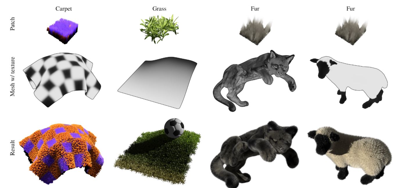
Modeling complex materials, such as fur, grass, or fabrics, is one such challenging scenario. NeRF-Tex addresses this challenge by utilizing a neural network to represent a small piece of fuzzy geometry. In order to create an object, an artist would model a base triangle mesh and instantiate the NeRF texture over its surface to create a volumetric layer with the desired structure, e.g., to dress a triangle mesh of a cat with fur.
Classical textures have traditionally been used to handle surface appearance. In contrast, NeRF Tex handles entire classes of volumetric appearance. For instance, a single NeRF texture could handle cases ranging from short, dark fur to bright, curly fibers. The spatial variations of the material are encoded using classical textures, effectively elevating these to control a volumetric structure above the surface.
Another great advantage of using neural networks for representing complex materials is the ability to perform level-of-detail rendering. The neural network is trained to reproduce filtered results to combat aliasing artifacts that classical primitives, like curves and triangles, are susceptible to.
The development of NeRF-Tex has been spearheaded by Hendrik Baatz and was done in collaboration with ETH Zurich and Disney Research|Studios. We are all excited about the potential of neural primitives for material modeling. More research and development is needed, but they could become powerful tools in offline and real-time production for creating photorealistic appearances in the future.
Efficient DGX System Sharing for Data Science Teams NVIDIA DGX is the universal system for AI and Data Science infrastructure. Hence, many organizations have incorporated DGX systems into their data centers for their data scientists and developers. The number of people running on these systems varies, from small teams of one to five people, to … Continued
Efficient DGX System Sharing for Data Science Teams
NVIDIA DGX is the universal system for AI and Data Science infrastructure. Hence, many organizations have incorporated DGX systems into their data centers for their data scientists and developers. The number of people running on these systems varies, from small teams of one to five people, to much larger teams of tens or maybe even hundreds of users. In this post we demonstrate how even a single DGX system can be efficiently utilized by multiple users. The focus in this blog is not on large DGX POD clusters. Rather, depending on the use cases, the deployment scale might be just one to several systems.
The deployment is managed via DeepOps toolkit, an open-source repository for common cluster management tasks. Using DeepOps organizations can customize features and scalability that are appropriate for their cluster and team sizes. Even when sharing just one DGX, users will have the capabilities and features of a rich cluster API to dynamically and efficiently run their workloads. That said, please note that DeepOps will require commitment from an organization’s DevOps professionals to tweak and maintain the underlying deployment. It is free and open-source software without support from NVIDIA.
DeepOps cluster API
DeepOps covers setting up login nodes, management, monitoring, Kubernetes, Slurm, and even storage provisioning. Figure 1 illustrates a cluster with the DeepOps components.
Figure 1. DeepOps view of cluster management.
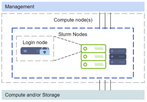
The above setup with management nodes, Kubernetes and other components would require additional servers, either physical or virtual, to be provisioned. Some organizations might acquire just DGX systems, and even with one node this will be sufficient without additional servers to set up a multi-user environment. However, deploying Kubernetes with just one node is not supported. Refer to the “Zero to Data Science” blog on deploying Kubernetes. We will rely on Slurm for the cluster resource manager and scheduling. This limited scope is illustrated in Figure 2.
Figure 2. Simplified cluster management with one of the compute nodes functioning as a login node.
Since the major difference in this setup is that one of the compute nodes functions as a login node, a few modifications are recommended. The GPU devices are restricted from regular login ssh sessions. When a user needs to run something on a GPU they would need to start a Slurm job session. The requested GPUs would then be available within the Slurm job session.
Additionally, in multi-user environments one typically wants to restrict elevated privileges for regular users. Rootless docker is used with the Slurm setup to avoid granting elevated rights to end users running containers. Rootless docker solves a couple problems. 1. The users can work in a familiar fashion with docker and NGC containers; 2. There is no need to add users to a privileged docker group; 3. The rootless docker sessions will be constrained to the Slurm job resources (privileged docker can bypass Slurm allocation constraints whereas rootless cannot).
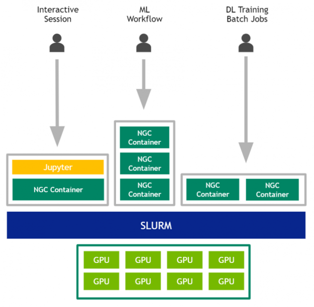
In summary the users would interact with the GPUs per Figure 3.
Figure 3. Multi-user team sharing a DGX system and its GPUs for various workloads.
The DeepOps Slurm deployment instructions for single node setup are available on github.In this blog the platform is DGX. The recommended setup is the latest DGX OS with the latest firmware updates. A pristine freshly imaged DGX is preferred. Refer to the NVIDIA enterprise support portal for the latest DGX updates as well as the DGX release notes.
The steps shown in this document should be executed by a user with sudo privileges, such as the user created during initial DGX OS installation.
This will install Ansible and other prerequisite utilities for running deepops.
$ ./scripts/setup.sh
3. Edit config and options.
After running the setup script in step 2, a copy of “config.example” directory will be made to “config” directory. When one of the compute nodes also functions as a login node a few special configurations have to be set.
a. Configuring inventory “config/inventory”
Let a host be named “gpu01” (DGX-1 with 8 GPUs) with an ssh reachable ip address of “192.168.1.5” and some admin user “dgxuser”. Then a single node config would look like this:
$ vi config/inventory
[all]
gpu01     ansible_host=192.168.1.5

[slurm-master]
gpu01

[slurm-node]
gpu01

[all:vars]
# SSH User
ansible_user=dgxuser
ansible_ssh_private_key_file='~/.ssh/id_rsa'
If the machine has a different hostname (i.e. not gpu01), then use the desired host name. Running the deployment will change the hostname to what is set in the inventory file. Otherwise one can set the “deepops_set_hostname” var in “config/group_vars/all.yml” (refer to DeepOps Ansible configuration options).
Depending on how the ssh is configured on the cluster one might have to generate a passwordless private key. Leave the password blank when prompted:
b. Configuring “config/group_vars/slurm-cluster.yml”
We need to add users to Slurm configuration for the ability to ssh as local users. This is needed when a compute node also functions as a login node. Additionally, set the singularity install option (which is “no” by default). Singularity can be used to run containers and it will be used to set up rootless options as well. Do not set up a default NFS with single node deployment.
Note: After deployment new users have to be manually added to “/etc/localusers” and “/etc/slurm/localusers.backup” on the node that functions as a login node.
4. Verify the configuration.
Check that ansible can run successfully and reach hosts. Run the hostname utility on “all” nodes. The “all” refers to the section in the “config/inventory” file. $ ansible all --connection=local -m raw -a "hostname"
For non-local setup does not set a connection to local. This requires ssh config to be set up properly in the “config/inventory”. Check connections via. $ ansible all -m raw -a "hostname"
5. Install Slurm.
When running Ansible, specify “–forks=1” so that Ansible does not perform potentially conflicting operations required for a slurm-master and slurm-node in parallel on the same node.The “–forks=1” option will ensure that the installation steps are serial.
For non-local installs do not set connection to local. The forks option is still required.
# NOTE: If SSH requires a password, add: `-k`
# NOTE: If sudo on remote machine requires a password, add: `-K`
# NOTE: If SSH user is different than current user, add: `-u ubuntu`
$ ansible-playbook -K --forks=1 -l slurm-cluster playbooks/slurm-cluster.yml
During Slurm playbook reboot is usually done twice:
Once after installing the NVIDIA driver, because the driver sometimes requires a reboot to load correctly.
Once after setting some grub options used for Slurm compute nodes to configure cgroups correctly, because of modification to the kernel command line.
The above reboot sequence cannot be automated when the compute and login nodes are on the same system. The recommended approach is to reboot manually when prompted and then run Ansible again. Setting “slurm_login_on_compute” to true, the slurm-cluster playbook will restrict GPUs in ssh sessions on the slurm-master by running the following command:
The reasoning for hiding GPUs in regular ssh sessions is that we want to avoid having users run a compute task on the GPUs without a Slurm job. If you desire to use docker within slurm then also install rootless docker after slurm deployment via playbook:
The admin users can access the GPUs that are restricted from regular ssh login sessions. This could be useful in situations when maybe GPU firmware needs to be updated. Let “dgxuser” be an admin user, they would access GPUs via command:
Refer to official Slurm documentation for additional admin configurations and options. Typical Slurm options one might want to configure are time limits on jobs, accounts, qos and priority settings, etc.
Monitoring GPUs
Refer to DeepOps documentation regarding how monitoring is configured and deployed on the Slurm cluster.
The grafana dashboard will be available at the ip address of the manager node on port 3000 (with above config http://192.168.1.5:3000). Either open the url at the manager node’s ip address or tunnel. SSH tunnel example:
$ ssh -L localhost:3000:localhost:3000 dgxuser@192.168.1.5
# open url:
http://127.0.0.1:3000/
On RHEL the grafana service might need to be exposed via firewall-cmd.
After Slurm is deployed, the users can now request GPUs and run containers. The following examples demonstrate the working pattern for a multi-user team sharing a single DGX system.
Initial SSH to Login Node
Let the ip address of the login system be “192.168.1.5” and user “testuser”. They would ssh to the system as follows:
$ ssh testuser@192.168.1.5
testuser@192.168.1.5's password:
Welcome to NVIDIA DGX Server Version 5.0.0 (GNU/Linux 5.4.0-52-generic x86_64)

  System information as of Wed 09 Dec 2020 10:16:09 PM UTC

  System load:  0.11                Processes:                 908
  Usage of /:   12.9% of 437.02GB   Users logged in:           2
  Memory usage: 1%                  IPv4 address for docker0:  172.17.0.1
  Swap usage:   0%                  IPv4 address for enp1s0f0: 192.168.1.5
  Temperature:  47.0 C

The system has 0 critical alerts and 5 warnings. Use 'sudo nvsm show alerts' for more details.

Last login: Tue Dec  1 00:01:32 2020 from 172.20.176.144
login-session:$
At this point, the tester would not be able to run anything on GPUs. This is because the GPUs are not available to the user via the initial ssh login session.
login-session:$ nvidia-smi -L
No devices found.
It might be useful just in case to ssh again in another terminal window. The second login session could be used for monitoring jobs or to perform auxiliary tasks, whereas the first session would be used to launch jobs interactively (more on this in the following sections).
Allocating GPUs
To request a GPU the testuser must first run a Slurm command with GPU allocation. Example:
compute-session:$ nvidia-smi -L
GPU 0: Tesla P100-SXM2-16GB (UUID: GPU-61ba3c7e-584a-7eb4-d993-2d0b0a43b24f)
The job allocations details in Slurm can be viewed in another pane (such as one of the tmux panes in the login session without GPU access) via “squeue” command and details of the job can be viewed via “scontrol”.
             JOBID PARTITION     NAME     USER ST       TIME  NODES NODELIST(REASON)
               106     batch     bash testuser  R       3:34      1 gpu01
DeepOps deploys Slurm with “pam_slurm_adopt” such that ssh sessions are permitted and adopted to allocated nodes. What that means is once a user has a Slurm job, additional ssh sessions will be adopted to the job. Proceeding with the above example, let us assume that job 106 is running. If the testuser were to make another ssh connection it would be adopted into job 106. If there were multiple jobs the default behaviour would be adopted into the latest job.
Such ssh sessions are useful in various use cases: monitoring, debugging, additional launch commands, and so on. These adopted ssh sessions are automatically terminated when the corresponding Slurm job ends. The above scenario is also why it is convenient to use tmux with the initial ssh session.
Running containers
NVIDIA provides many AI, HPC, and Data Science containers. These are hosted on NGC. Take advantage of these GPU optimized containers. DeepOps enables running containers with several containerization alternatives: docker, singularity, and enroot with pyxis.
Rootless Docker
Docker remains the de facto industry standard for containerization. Docker is very easy to work with when building and extending containers. NGC and many other data science software stacks are distributed as docker containers. Fortunately, it is straightforward to incorporate rootless docker with Slurm. The reason for using rootless docker is that we want to avoid granting elevated privileges to users unnecessarily.
DeepOps sets up rootless docker as a module package. Environment modules are a popular way to set up cluster wide software for sharing. On a side note, DeepOps can set up easybuild or spack to manage environment modules and packages. The workflow with rootless docker is as follows: 1. A user starts a slurm job; 2. Module load the rootless docker package; 3. Start rootless docker daemon; 4. Work with docker containers per regular docker workflow. The following examples will illustrate the commands.
The “–gpus=all” refers to all GPUs that are scheduled in the Slurm session, not all GPUs on the host. This could be placed in a script and run with srun or sbatch. Example:
The Slurm constraints are enforced for rootless docker. This can be verified by starting the container in an interactive slurm session and checking the number of GPUs and CPUs available.
Rootless docker runs via user namespace remapping. Files created are owned by the user, and within the container a user would not have write/execute permissions to filesystem or executables that the user already does not have permission to outside of the container. Thus user privileges are not elevated within Slurm when using rootless docker.
A user can explicitly stop the rootless docker daemon with “stop_rootless_docker.sh” script, or just exit the Slurm session. Upon ending a slurm session, processes in the session are killed and therefore the user’s rootless docker process will end.
These scripts “start_rootless_docker.sh” and “stop_rootless_docker.sh” appear on a user’s path after loading the rootless docker module.
Enroot and singularity
Although beyond the scope of this blog, enroot and singularity could also be deployed via DeepOps. These are especially useful for multi-node jobs if running on more than one DGX system. The examples below though are for single node jobs.
The pyxis+enroot is invoked via option “–container-image” to run the container. Refer to enroot and pyxis documentation for further details.
Singularity could be used in a similar fashion to enroot. Using singularity it is typically more efficient to convert the docker container to singularity format (“*.sif”) prior to running the job. Don’t forget the “–nv” option for GPUs. Example:
Refer to singularity documentation for further details. Building containers with singularity is permitted to non-privileged users via the “–fakeroot” option.
Enroot and Singularity excel at running containerized multinode jobs, which is somewhat difficult and less convenient to do using docker on Slurm. The focus of the blog is on single node DeepOps deployment, but if multinode containerized jobs on Slurm are of interest consider enroot and singularity for that task.
Conclusion
DeepOps aims to make managing GPU clusters flexible and scalable. Various organizations ranging from enterprises to small businesses, startups, and educational institutions, can adopt and deploy DeepOps features relevant to their teams. Admins have tools at their disposal to manage GPUs effectively. Meanwhile, users can collaborate and work productively and efficiently on shared GPU resources.
Get started with DeepOps and refer to the tips in this blog to work productively with your GPUs and DGX systems.
Posted by Mauricio Delbracio, Research Scientist and Sungjoon Choi, Software Engineer, Google Research
Despite recent leaps in imaging technology, especially on mobile devices, image noise and limited sharpness remain two of the most important levers for improving the visual quality of a photograph. These are particularly relevant when taking pictures in poor light conditions, where cameras may compensate by increasing the ISO or slowing the shutter speed, thereby exacerbating the presence of noise and, at times, increasing image blur. Noise can be associated with the particle nature of light (shot noise) or be introduced by electronic components during the readout process (read noise). The captured noisy signal is then processed by the camera image processor (ISP) and later may be further enhanced, amplified, or distorted by a photographic editing process. Image blur can be caused by a wide variety of phenomena, from inadvertent camera shake during capture, an incorrect setting of the camera’s focus (automatic or not), or due to the finite lens aperture, sensor resolution or the camera’s image processing.
It is far easier to minimize the effects of noise and blur within a camera pipeline, where details of the sensor, optical hardware and software blocks are understood. However, when presented with an image produced from an arbitrary (possibly unknown) camera, improving noise and sharpness becomes much more challenging due to the lack of detailed knowledge and access to the internal parameters of the camera. In most situations, these two problems are intrinsically related: noise reduction tends to eliminate fine structures along with unwanted details, while blur reduction seeks to boost structures and fine details. This interconnectedness increases the difficulty of developing image enhancement techniques that are computationally efficient to run on mobile devices.
Today, we present a new approach for camera-agnostic estimation and elimination of noise and blur that can improve the quality of most images. We developed a pull-push denoising algorithm that is paired with a deblurring method, called polyblur. Both of these components are designed to maximize computational efficiency, so users can successfully enhance the quality of a multi-megapixel image in milliseconds on a mobile device. These noise and blur reduction strategies are critical components of the recent Google Photos editor updates, which includes “Denoise” and “Sharpen” tools that enable users to enhance images that may have been captured under less than ideal conditions, or with older devices that may have had more noisy sensors or less sharp optics.
A demonstration of the “Denoise” and “Sharpen” tools now available in the Google Photos editor.
How Noisy is An Image? In order to accurately process a photographic image and successfully reduce the unwanted effects of noise and blur, it is vitally important to first characterize the types and levels of noise and blur found in the image. So, a camera-agnostic approach for noise reduction begins by formulating a method to gauge the strength of noise at the pixel level from any given image, regardless of the device that created it. The noise level is modeled as a function of the brightness of the underlying pixel. That is, for each possible brightness level, the model estimates a corresponding noise level in a manner agnostic to either the actual source of the noise or the processing pipeline.
To estimate this brightness-based noise level, we sample a number of small patches across the image and measure the noise level within each patch, after roughly removing any underlying structure in the image. This process is repeated at multiple scales, making it robust to artifacts that may arise from compression, image resizing, or other non-linear camera processing operations.
The two segments on the left illustrate signal-dependent noise present in the input image (center). The noise is more prominent in the bottom, darker crop and is unrelated to the underlying structure, but rather to the light level. Such image segments are sampled and processed to generate the spatially-varying noise map (right) where red indicates more noise is present.
Reducing Noise Selectively with a Pull-Push Method We take advantage of self-similarity of patches across the image to denoise with high fidelity. The general principle behind such so-called “non-local” denoising is that noisy pixels can be denoised by averaging pixels with similar local structure. However, these approaches typically incur high computational costs because they require a brute force search for pixels with similar local structure, making them impractical for on-device use. In our “pull-push” approach1, the algorithmic complexity is decoupled from the size of filter footprints thanks to effective information propagation across spatial scales.
The first step in pull-push is to build an image pyramid (i.e., multiscale representation) in which each successive level is generated recursively by a “pull” filter (analogous to downsampling). This filter uses a per-pixel weighting scheme to selectively combine existing noisy pixels together based on their patch similarities and estimated noise, thus reducing the noise at each successive, “coarser” level. Pixels at coarser levels (i.e., with lower resolution) pull and aggregate only compatible pixels from higher resolution, “finer” levels. In addition to this, each merged pixel in the coarser layers also includes an estimated reliability measure computed from the similarity weights used to generate it. Thus, merged pixels provide a simple per-pixel, per-level characterization of the image and its local statistics. By efficiently propagating this information through each level (i.e., each spatial scale), we are able to track a model of the neighborhood statistics for increasingly larger regions in a multiscale manner.
After the pull stage is evaluated to the coarsest level, the “push” stage fuses the results, starting from the coarsest level and generating finer levels iteratively. At a given scale, the push stage generates “filtered” pixels following a process similar to that of the pull stage, but going from coarse to finer levels. The pixels at each level are fused with those of coarser levels by doing a weighted average of same-level pixels along with coarser-level filtered pixels using the respective reliability weights. This enables us to reduce pixel noise while preserving local structure, because only average reliable information is included. This selective filtering and reliability (i.e. information) multiscale propagation is what makes push-pull different from existing frameworks.
This series of images shows how filtering progresses through the pull-push process. Coarser level pixels pull and aggregate only compatible pixels from finer levels, as opposed to the traditional multiscale approaches using a fixed (non-data dependent) kernel. Notice how the noise is reduced throughout the stages.
The pull-push approach has a low computational cost, because the algorithm to selectively filter similar pixels over a very large neighborhood has a complexity that is only linear with the number of image pixels. In practice, the quality of this denoising approach is comparable to traditional non-local methods with much larger kernel footprints, but operates at a fraction of the computational cost.
Image enhanced using the pull-push denoising method.
How Blurry Is an Image? An image with poor sharpness can be thought of as being a more pristine latent image that was operated on by a blur kernel. So, if one can identify the blur kernel, it can be used to reduce the effect. This is referred to as “deblurring”, i.e., the removal or reduction of an undesired blur effect induced by a particular kernel on a particular image. In contrast, “sharpening” refers to applying a sharpening filter, built from scratch and without reference to any particular image or blur kernel. Typical sharpening filters are also, in general, local operations that do not take account of any other information from other parts of the image, whereas deblurring algorithms estimate the blur from the whole image. Unlike arbitrary sharpening, which can result in worse image quality when applied to an image that is already sharp, deblurring a sharp image with a blur kernel accurately estimated from the image itself will have very little effect.
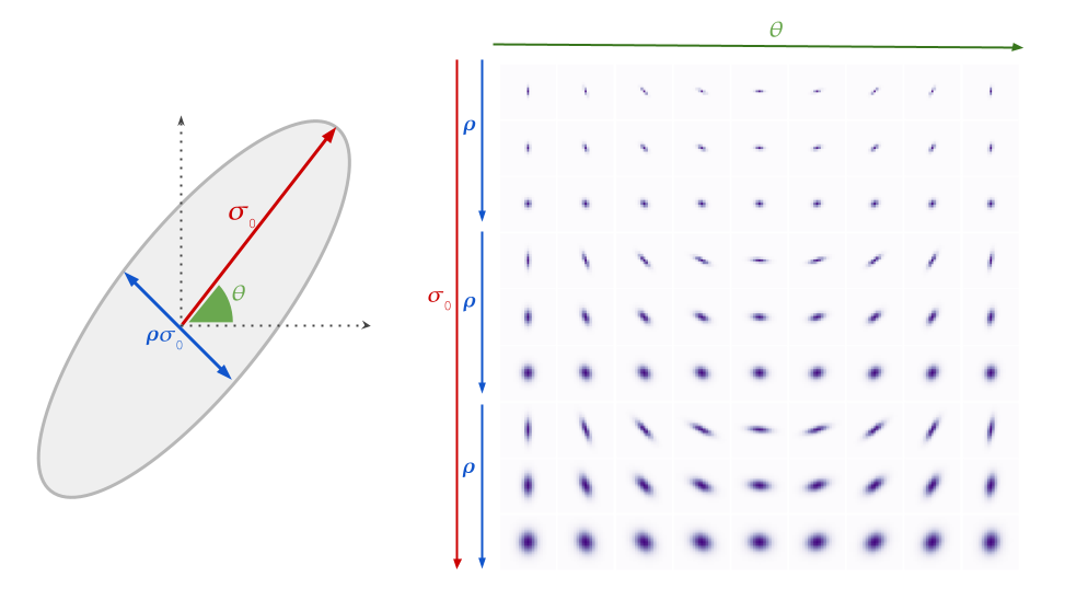
We specifically target relatively mild blur, as this scenario is more technically tractable, more computationally efficient, and produces consistent results. We model the blur kernel as an anisotropic (elliptical) Gaussian kernel, specified by three parameters that control the strength, direction and aspect ratio of the blur.
Gaussian blur model and example blur kernels. Each row of the plot on the right represents possible combinations of σ0, ρ and θ. We show three different σ0 values with three different ρ values for each.
Computing and removing blur without noticeable delay for the user requires an algorithm that is much more computationally efficient than existing approaches, which typically cannot be executed on a mobile device. We rely on an intriguing empirical observation: the maximal value of the image gradient across all directions at any point in a sharp image follows a particular distribution. Finding the maximum gradient value is efficient, and can yield a reliable estimate of the strength of the blur in the given direction. With this information in hand, we can directly recover the parameters that characterize the blur.
Polyblur: Removing Blur by Re-blurring To recover the sharp image given the estimated blur, we would (in theory) need to solve a numerically unstable inverse problem (i.e., deblurring). The inversion problem grows exponentially more unstable with the strength of the blur. As such, we target the case of mild blur removal. That is, we assume that the image at hand is not so blurry as to be beyond practical repair. This enables a more practical approach — by carefully combining different re-applications of an operator we can approximate its inverse.
Mild blur, as shown in these examples, can be effectively removed by combining multiple applications of the estimated blur.
This means, rather counterintuitively, that we can deblur an image by re-blurring it several times with the estimated blur kernel. Each application of the (estimated) blur corresponds to a first order polynomial, and the repeated applications (adding or subtracting) correspond to higher order terms in a polynomial. A key aspect of this approach, which we call polyblur, is that it is very fast, because it only requires a few applications of the blur itself. This allows it to operate on megapixel images in a fraction of a second on a typical mobile device. The degree of the polynomial and its coefficients are set to invert the blur without boosting noise and other unwanted artifacts.
The deblurred image is generated by adding and subtracting multiple re-applications of the estimated blur (polyblur).
Integration with Google Photos The innovations described here have been integrated and made available to users in the Google Photos image editor in two new adjustment sliders called “Denoise” and “Sharpen”. These features allow users to improve the quality of everyday images, from any capture device. The features often complement each other, allowing both denoising to reduce unwanted artifacts, and sharpening to bring clarity to the image subjects. Try using this pair of tools in tandem in your images for best results. To learn more about the details of the work described here, check out our papers on polyblur and pull-push denoising. To see some examples of the effect of our denoising and sharpening up close, have a look at the images in this album.
Acknowledgements The authors gratefully acknowledge the contributions of Ignacio Garcia-Dorado, Ryan Campbell, Damien Kelly, Peyman Milanfar, and John Isidoro. We are also thankful for support and feedback from Navin Sarma, Zachary Senzer, Brandon Ruffin, and Michael Milne.
1 The original pull-push algorithm was developed as an efficient scattered data interpolation method to estimate and fill in the missing pixels in an image where only a subset of the pixels are specified. Here, we extend its methodology and present a data-dependent multiscale algorithm for denoising images efficiently. ↩
NVIDIA Omniverse has expanded to address the scientific visualization community with aConnector to Kitware ParaView, one of the world’s most popular scientific visualization applications.
Now available by downloading Omniverse Open Beta, the Omniverse ParaView Connector enables researchers to boost their productivity and speed their discoveries. Large datasets no longer need to be downloaded and exchanged, and colleagues can get instantaneous feedback as Omniverse users can work in the same workspace in the cloud.
ParaView, an open-source, multi-platform data analysis and visualization application, enables users to quickly build visualizations so they can analyze and explore their data using qualitative and quantitative techniques. Researchers use ParaView to analyze massive datasets, and typically run the application on supercomputers to analyze datasets of petascale, as well as on laptops for smaller data.
The Omniverse ParaView Connector provides researchers with a toolkit that allows them to send and live sync their models to an NVIDIA Omniverse Nucleus Server, or alternatively locally output them to USD, with OpenVDB in case of volumes. This enables the user to edit and sync their ParaView data with any Omniverse Connect applications, or just import it into applications supporting USD or OpenVDB.
Simulating fuel injection in a combustion engine
Omniverse ParaView Connector works in multiple deployments and environments, including headless EGL Kitware ParaView servers, multi-node MPI environments, and python environments. The Connector adds to ParaView a render view, two filters, and an additional tab in ParaView’s settings dialog for global configuration.
For more information, see the Install Instructions for a walkthrough in configuring and using the connector, and check out the additional features available, including:

 Learn how NVIDIA NGC and NVIDIA Clara (NVIDIA’s healthcare AI Platform) can help accelerate medical imaging workflows.
 NVIDIA Inception member, IPMD won the Touchless Experience category of Texas Children’s Hospital Healthcare Hackathon with its Project M emotional AI solution.
 NVIDIA researchers collaborated with ETH Zurich and Disney Research|Studios on a new paper, “NeRF-Tex: Neural Reflectance Field Textures” that will be presented at the Eurographics Symposium on Rendering (EGSR) June 29 – July 2, 2021. The paper introduces a new modeling primitive: neural reflectance field textures, or NeRF-Tex for short. NeRF-Tex is inspired by recent …
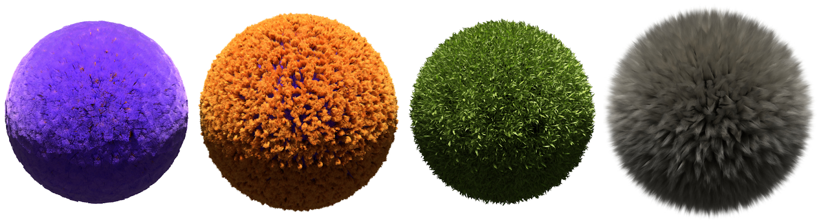
 Efficient DGX System Sharing for Data Science Teams NVIDIA DGX is the universal system for AI and Data Science infrastructure. Hence, many organizations have incorporated DGX systems into their data centers for their data scientists and developers. The number of people running on these systems varies, from small teams of one to five people, to …
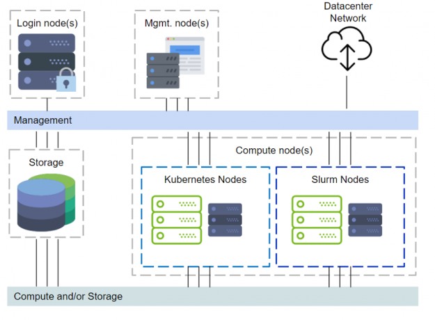


 NVIDIA Omniverse has expanded to address the scientific visualization community with aConnector to Kitware ParaView, one of the world’s most popular scientific visualization applications.