Is visualizing data a necessity to solving the problems?
Is there an age requirement?
Does the exam normally take the full 5 hours?
submitted by /u/Sad_Combination9971
[visit reddit] [comments]
 DataBloom
Is visualizing data a necessity to solving the problems?
Is there an age requirement?
Does the exam normally take the full 5 hours?
submitted by /u/Sad_Combination9971
[visit reddit] [comments]
I (dumb) thought anaconda would automatically choose the proper version for the type of chip, turns out I have been using the intel-based python all this time instead of the native version.
/Users/x/opt/anaconda3/envs/ml/bin/python: Mach-O 64-bit executable x86_64
It should say:
... Mach-O 64-bit executable arm64
Now, it is normal to use the intel based version if not already updated to native silicon? I guess I’m just missing out on M1 performance?
From my understanding, the only way to download the native Python 3.9X versions is through homebrew / miniforge: TLDR. Is it worth updating, especially considering I’m starting to use TensorFlow, etc. for ML? Also, what happens to all my current envs and packages I have in (the current, intel based ) anaconda if I switch to Miniforge? Do they all translate, or what happens to the packages not optimised for arm64?
Or is the performance not life changing at all and I should save myself headaches and keep using TensorFlow 2.0.0 on the intel-based anaconda / python 3.6?
submitted by /u/capital-man
[visit reddit] [comments]
 Simulated or synthetic data generation is an important emerging trend in the development of AI tools. Classically, these datasets can be used to address low-data problems or edge-case scenarios that might now be present in available real-world datasets. Emerging applications for synthetic data include establishing model performance levels, quantifying the domain of applicability, and next-generation … Continued
Simulated or synthetic data generation is an important emerging trend in the development of AI tools. Classically, these datasets can be used to address low-data problems or edge-case scenarios that might now be present in available real-world datasets.
Emerging applications for synthetic data include establishing model performance levels, quantifying the domain of applicability, and next-generation systems engineering, where AI models and sensors are designed in tandem.
Blender is a common and compelling tool for generating these datasets. It is free to use and open source but, just as important, it is fully extensible through a powerful Python API. This feature of Blender has made it an attractive option for visual image rendering. As a result, it has been used extensively for this purpose, with 18+ rendering engine options to choose from.
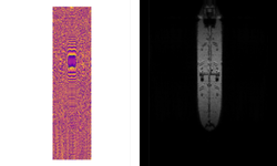
Rendering engines integrated into Blender, such as Cycles, often come with tightly integrated GPU support, including state-of-the-art NVIDIA RTX support. However, if high performance levels are required outside of a visual rendering engine, such as the render of a synthetic SAR image, the Python environment can be too sluggish for practical applications. One option to accelerate this code is to use the popular Numba package to precompile portions of the Python code into C. This still leaves room for improvement, however, particularly when it comes to the adoption of leading GPU architectures for scientific computing.
GPU capabilities for scientific computing can be available from directly within Blender, allowing for simple unified tools that leverage Blender’s powerful geometry creation capabilities as well as cutting-edge computing environments. As of the recent changes in Blender 2.83+, this can be done using CuPy, a GPU-accelerated Python library devoted to array calculations, directly from within a Python script.
In line with these ideas, the following tutorial compares two different ways of accelerating matrix multiplication. The first approach uses Python’s Numba compiler while the second approach uses the NVIDIA GPU-compute API, CUDA. Implementation of these approaches can be found in the rleonard1224/matmul GitHub repo, along with a Dockerfile that sets up an anaconda environment from which CUDA-accelerated Blender Python scripts can be run.
As a precursor to discussing the different approaches used to accelerate matrix multiplication, we briefly review matrix multiplication itself.
For the product of two matrices ![[A cdot B]](https://s0.wp.com/latex.php?latex=%5BA+%5Ccdot+B%5D&bg=ffffff&fg=000&s=0&c=20201002)
![[A]](https://s0.wp.com/latex.php?latex=%5BA%5D&bg=ffffff&fg=000&s=0&c=20201002)
![[B]](https://s0.wp.com/latex.php?latex=%5BB%5D&bg=ffffff&fg=000&s=0&c=20201002)
then is a matrix with ![[m]](https://s0.wp.com/latex.php?latex=%5Bm%5D&bg=ffffff&fg=000&s=0&c=20201002) rows and
rows and ![[n]](https://s0.wp.com/latex.php?latex=%5Bn%5D&bg=ffffff&fg=000&s=0&c=20201002) columns, that is, an
columns, that is, an ![[m times n]](https://s0.wp.com/latex.php?latex=%5Bm+%5Ctimes+n%5D&bg=ffffff&fg=000&s=0&c=20201002) matrix. is an
matrix. is an ![[n times p]](https://s0.wp.com/latex.php?latex=%5Bn+%5Ctimes+p%5D&bg=ffffff&fg=000&s=0&c=20201002) matrix.
matrix.![[C = A cdot B]](https://s0.wp.com/latex.php?latex=%5BC+%3D+A+%5Ccdot+B%5D&bg=ffffff&fg=000&s=0&c=20201002) results in an
results in an ![[m times p]](https://s0.wp.com/latex.php?latex=%5Bm+%5Ctimes+p%5D&bg=ffffff&fg=000&s=0&c=20201002) matrix.
matrix.If the first element in each row and each column of ![[C]](https://s0.wp.com/latex.php?latex=%5BC%5D&bg=ffffff&fg=000&s=0&c=20201002)
![[C[i,j]]](https://s0.wp.com/latex.php?latex=%5BC%5Bi%2Cj%5D%5D&bg=ffffff&fg=000&s=0&c=20201002)
The Numba compiler can be applied to a function in a Python script by using the numba.jit decorator. By precompilation into C, the use of the numba.jit decorator significantly reduces the run times of loops when used in Python code. Because matrix multiplication translated directly into code requires nested for loops, use of the numba.jit decorator significantly reduces the run times of a matrix multiplication function written in Python. The matmulnumba.py Python script implements matrix multiplication and uses the numba.jit decorator.
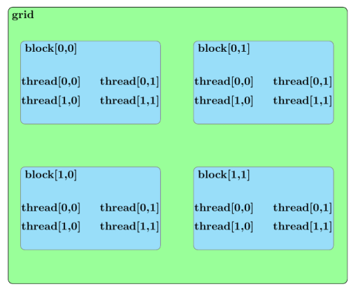
Before we discuss an approach to accelerate matrix multiplication using CUDA, we should broadly outline the parallel structure of a CUDA kernel launch. All parallel processes within a kernel launch belong to a grid. A grid is composed of an array of blocks and each block is composed of an array of threads. The threads within a grid compose the fundamental parallel processes launched by a CUDA kernel. Figure 2 outlines a sample parallel structure of this kind.
Now that this summary of the parallel structure of a CUDA kernel launch is spelled out, the approach used to parallelize matrix multiplication in the matmulcuda.py Python script can be described as follows.
Suppose the following are to be calculated by a CUDA kernel grid composed of a 2D array of blocks with each block composed of a 1D array of threads:
and matrix and matrix and matrix Also, further assume the following:
![[textrm{nblocksx}]](https://s0.wp.com/latex.php?latex=%5B%5Ctextrm%7Bnblocksx%7D%5D&bg=ffffff&fg=000&s=0&c=20201002) ) is greater than or equal to (
) is greater than or equal to (![[textrm{nblocksx} geq m]](https://s0.wp.com/latex.php?latex=%5B%5Ctextrm%7Bnblocksx%7D+%5Cgeq+m%5D&bg=ffffff&fg=000&s=0&c=20201002) ).
).![[textrm{nblocksy}]](https://s0.wp.com/latex.php?latex=%5B%5Ctextrm%7Bnblocksy%7D%5D&bg=ffffff&fg=000&s=0&c=20201002) ) is greater than or equal to
) is greater than or equal to ![[p]](https://s0.wp.com/latex.php?latex=%5Bp%5D&bg=ffffff&fg=000&s=0&c=20201002) (
(![[textrm{nblocksy} geq p]](https://s0.wp.com/latex.php?latex=%5B%5Ctextrm%7Bnblocksy%7D+%5Cgeq+p%5D&bg=ffffff&fg=000&s=0&c=20201002) ).,
).,![[textrm{nthreads}]](https://s0.wp.com/latex.php?latex=%5B%5Ctextrm%7Bnthreads%7D%5D&bg=ffffff&fg=000&s=0&c=20201002) ) is greater than or equal to (
) is greater than or equal to (![[textrm{nthreads} geq n]](https://s0.wp.com/latex.php?latex=%5B%5Ctextrm%7Bnthreads%7D+%5Cgeq+n%5D&bg=ffffff&fg=000&s=0&c=20201002) ).
).The elements of the matrix product
You can obtain further parallel enhancement by assigning, to each thread of the block to which
To avoid a race condition, the summing of these atomicAdd function. The atomicAdd function signature consists of a pointer as the first input and a numerical value as the second input. The definition adds the numerical value input to the value pointed to by the first input and later stores this sum in the location pointed to by the first input.
Assume that the elements of ![[textrm{tid}(i,j)]](https://s0.wp.com/latex.php?latex=%5B%5Ctextrm%7Btid%7D%28i%2Cj%29%5D&bg=ffffff&fg=000&s=0&c=20201002)
![[[i,j]]](https://s0.wp.com/latex.php?latex=%5B%5Bi%2Cj%5D%5D&bg=ffffff&fg=000&s=0&c=20201002)
Figure 3 summarizes this parallel arrangement for the multiplication of two sample matrices of ![[2 times 2]](https://s0.wp.com/latex.php?latex=%5B2+%5Ctimes+2%5D&bg=ffffff&fg=000&s=0&c=20201002)
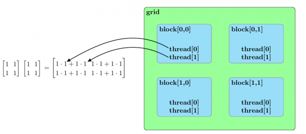
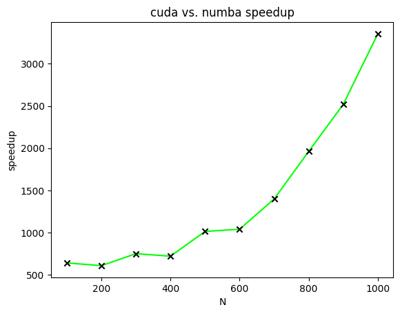
Figure 4 displays the speedups of CUDA-accelerated matrix multiplication relative to Numba-accelerated matrix multiplication for matrices of varying sizes. In this figure, speedups are plotted for the calculation of two ![[N times N]](https://s0.wp.com/latex.php?latex=%5BN+%5Ctimes+N%5D&bg=ffffff&fg=000&s=0&c=20201002)
![[N]](https://s0.wp.com/latex.php?latex=%5BN%5D&bg=ffffff&fg=000&s=0&c=20201002)
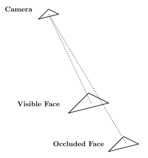
Given Blender’s role as a computer graphics tool, one relevant area of application suitable for CUDA acceleration relates to solving the visibility problem through ray tracing. The visibility problem can be broadly summarized as follows: A camera exists at some point in space and is looking at a mesh composed of, for instance, triangular elements. The goal of the visibility problem is to determine which mesh elements are visible to the camera and which are instead occluded by other mesh elements.
Ray tracing can be used to solve the visibility problem. A mesh whose visibility you are trying to determine is composed of
Each ray has an endpoint at a different mesh element. If a ray reaches its endpoint without being occluded by another mesh element, then the endpoint mesh element is visible from the camera. Figure 5 shows this procedure.
The nature of the use of ray tracing to solve the visibility problem makes it an ![[mathcal{O}(N^{2})]](https://s0.wp.com/latex.php?latex=%5B%5Cmathcal%7BO%7D%28N%5E%7B2%7D%29%5D&bg=ffffff&fg=000&s=0&c=20201002)
This post described two different approaches for how to accelerate matrix multiplication. The first approach used the Numba compiler to decrease the overhead associated with loops in Python code. The second approach used CUDA to parallelize matrix multiplication. A speed comparison demonstrated the effectiveness of CUDA in accelerating matrix multiplication.
Because the CUDA-accelerated code described earlier can be run as a Blender Python script, any number of algorithms can be accelerated using CUDA from within a Blender Python environment. That greatly increases the effectiveness of Blender Python as a scientific computing tool.
If you have questions or comments, please comment below or contact us at info@rendered.ai.
 Learn about the latest GPU Operator releases which include support for multi-instance GPU Support, pre-installed NVIDIA drivers, Red Hat OpenShift 4.7, and more.
Reliably provisioning servers with GPUs in Kubernetes can quickly become complex as multiple components must be installed and managed to use GPUs. The GPU Operator, based on the Operator Framework, simplifies the initial deployment and management of GPU servers. NVIDIA, Red Hat, and others in the community have collaborated on creating the GPU Operator.
To provision GPU worker nodes in a Kubernetes cluster, the following NVIDIA software components are required:
These components should be provisioned before GPU resources are available to the cluster and managed during the cluster operation.
The GPU Operator simplifies both the initial deployment and management of the components by containerizing all components. It uses standard Kubernetes APIs for automating and managing these components, including versioning and upgrades. The GPU Operator is fully open source. It is available on NGC and as part of the NVIDIA EGX Stack and Red Hat OpenShift.
The latest GPU Operator releases, 1.6 and 1.7, include several new features:
Multi-Instance GPU (MIG) expands the performance and value of each NVIDIA A100 Tensor Core GPU. MIG can partition the A100 or A30 GPU into as many as seven instances (A100) or four instances (A30), each fully isolated with their own high-bandwidth memory, cache, and compute cores.
Without MIG, different jobs running on the same GPU, such as different AI inference requests, compete for the same resources, such as memory bandwidth. With MIG, jobs run simultaneously on different instances, each with dedicated resources for compute, memory, and memory bandwidth. This results in predictable performance with quality of service and maximum GPU utilization. Because simultaneous jobs can operate, MIG is ideal for edge computing use cases.
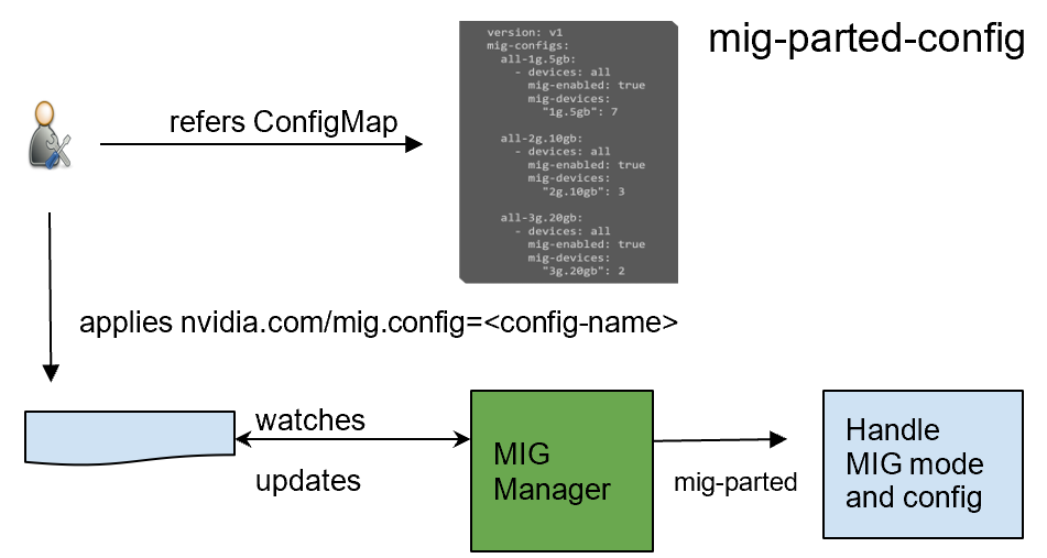
GPU Operator 1.7 added a new component called NVIDIA MIG Manager for Kubernetes, which runs as a DaemonSet and manages MIG mode and MIG configuration changes on each node. You can apply MIG configuration on the node by adding a label that indicates the predefined configuration name to be applied. After applying MIG configuration, GPU Operator automatically validates that MIG changes are applied as expected. For more information, see GPU Operator with MIG.
GPU Operator 1.7 now supports selectively installing NVIDIA Driver and Container Toolkit (container config) components. This new feature provides great flexibility for environments where the driver or nvidia-docker2 packages are preinstalled. These environments can now use GPU Operator for simplified management of other software components like Device Plugin, GPU Feature Discovery Plugin, DCGM Exporter for monitoring, or MIG Manager for Kubernetes.
Install command with only the drivers preinstalled:
 helm install --wait --generate-name
      nvidia/gpu-operator
      --set driver.enabled=false
Install command with both drivers and nvidia-docker2 preinstalled:
 helm install --wait --generate-name
      nvidia/gpu-operator
      --set driver.enabled=false
      --set toolkit.enabled=false
We continue our line of support for Red Hat OpenShift,
GPU Operator is an OpenShift certified operator. Through the OpenShift web console, you can install and start using the GPU Operator with only a few mouse clicks. Being a certified operator makes it significantly easier for you to use NVIDIA GPUs with Red Hat OpenShift.
We updated the GPU Driver version to include support for NVIDIA A40, A30, and A10.
The NVIDIA A40 delivers the data center-based solution that designers, engineers, artists, and scientists need for meeting today’s challenges. Built on the NVIDIA Ampere Architecture, the A40 combines the latest generation RT Cores, Tensor Cores, and CUDA Cores. It has 48 GB of graphics memory for unprecedented graphics, rendering, compute, and AI performance. From powerful virtual workstations accessible from anywhere, to dedicated render and compute nodes, the A40 is built to tackle the most demanding visual computing workloads from the data center.
For more information, see NVIDIA A40.
The NVIDIA A30 Tensor Core GPU is the most versatile mainstream compute GPU for AI inference and enterprise workloads. Tensor Cores with MIG combine with fast memory bandwidth in a low 165W power envelope, all in a PCIe form factor ideal for mainstream servers.
Built for AI inference at scale, A30 can also rapidly retrain AI models with TF32 as well as accelerate HPC applications using FP64 Tensor Cores. The combination of the NVIDIA Ampere Architecture Tensor Cores and MIG delivers speedups securely across diverse workloads, all powered by a versatile GPU enabling an elastic data center. The versatile A30 compute capabilities deliver maximum value for mainstream enterprises.
For more information, see NVIDIA A30.
The NVIDIA A10 Tensor Core GPU is the ideal GPU for mainstream media and graphics with AI. Second-generation RT Cores and third-generation Tensor Cores enrich graphics and video applications with powerful AI. NVIDIA A10 delivers a single-wide, full-height, full-length PCIe form factor and a 150W power envelope for dense servers.
Built for graphics, media, and cloud gaming applications with powerful AI capabilities, the NVIDIA A10 Tensor Core GPU can deliver rich media experiences. It delivers up to 4k for cloud gaming, with 2.5x the graphics and over 3x the inference performance compared to the NVIDIA T4 Tensor Core GPU.
For more information, see NVIDIA A10.
RuntimeClass provides you with the flexibility of choosing the container runtime configuration per Pod and then applying the default runtime configuration for all Pods on each node. With this support, you can specify the specific runtime configuration for Pods running GPU-accelerated workloads and choose other runtimes for generic workloads.
GPU Operator v1.7.0 now supports auto creation of nvidia RuntimeClass when default runtime is selected as containerd during installation. You can explicitly specify this RuntimeClass name when running applications consuming GPUs.
 apiVersion: node.k8s.io/v1beta1
 handler: nvidia
 kind: RuntimeClass
 metadata:
  labels:
    app.kubernetes.io/component: gpu-operator
  name: nvidia
To start using NVIDIA GPU Operator today, see the following resources:
 Is EVPN magic? As Arthur C Clarke said, any sufficiently advanced technology is indistinguishable from magic. On that premise, moving from a traditional layer 2 environment to VXLAN driven by EVPN has much of that same hocus-pocus feeling. To help demystify the sorcery, I aim to help users new to EVPN understand how EVPN works … Continued
Is EVPN magic? As Arthur C Clarke said, any sufficiently advanced technology is indistinguishable from magic. On that premise, moving from a traditional layer 2 environment to VXLAN driven by EVPN has much of that same hocus-pocus feeling.
To help demystify the sorcery, I aim to help users new to EVPN understand how EVPN works and how the control plane converges. In this post, I focus on basic layer 2 (L2) building blocks then work my way up to layer 3 (L3) connectivity and the control plane.
I use the reference topology as the cable plan and foundation to build your understanding of the traffic flow. The infrastructure tries to demystify a symmetric-mode EVPN environment using distributed gateways. All configurations are standardized using the production-ready automation and linked in the publicly available cumulus_ansible_modules GitLab repo.
To follow along, build your own Cumulus in the Cloud and deploy the following playbook:
~$ git clone https://gitlab.com/cumulus-consulting/goldenturtle/cumulus_ansible_modules.git

 Cloning into 'cumulus_ansible_modules'...
 remote: Enumerating objects: 822, done.
 remote: Counting objects: 100% (822/822), done.
 remote: Compressing objects: 100% (374/374), done.
 remote: Total 4777 (delta 416), reused 714 (delta 340), pack-reused 3955
 Receiving objects: 100% (4777/4777), 4.64 MiB | 22.64 MiB/s, done.
 Resolving deltas: 100% (2121/2121), done.

 ~$
 ~$ cd cumulus_ansible_modules/
 ~/cumulus_ansible_modules$ ansible-playbook -i inventories/evpn_symmetric/host playbooks/deploy.yml
Like any good protocol, EVPN has a robust process for exchanging information with its peers: message types. If you already know OSPF and the LSA messages, you can think of EVPN message types as similar. Each EVPN message type can carry a different kind of information about the EVPN traffic flow.
There are about five different message types. In this post, I focus on the two most popular types for now: Type 2 MAC and Type 2 MAC/IP information.
The easiest EVPN messages to understand are type 2. As mentioned earlier, type 2 routes contain MAC and MAC/IP mappings. To start off, inspect a type 2 entry at work. To do that, you can verify basic connectivity from leaf01 to the server01.
First, look at the bridge table to make sure that the MAC address of the switch has the correct mapping to the correct port for the server.
Get the Server01 MAC address:
cumulus@server01:~$ ip address show
 ...
 5: uplink:  mtu 9000 qdisc noqueue state UP group default qlen 1000
      link/ether 44:38:39:00:00:32 brd ff:ff:ff:ff:ff:ff
      inet 10.1.10.101/24 scope global uplink
      valid_lft forever preferred_lft forever
      inet6 fe80::4638:39ff:fe00:32/64 scope link
      valid_lft forever preferred_lft forever
Look at Leaf01’s bridge table to make sure the MAC address is mapped to the port that you expect. Cross reference it with LLDP:
cumulus@server01:~$ ip address show
 ...
 5: uplink:  mtu 9000 qdisc noqueue state UP group default qlen 1000
      link/ether 44:38:39:00:00:32 brd ff:ff:ff:ff:ff:ff
      inet 10.1.10.101/24 scope global uplink
      valid_lft forever preferred_lft forever
      inet6 fe80::4638:39ff:fe00:32/64 scope link
      valid_lft forever preferred_lft forever
 Look at Leaf01’s bridge table to make sure the MAC address is mapped to the port that you expect. Cross reference it with LLDP:

 cumulus@leaf01:mgmt:~$ net show bridge macs

 VLAN       Master  Interface  MAC                TunnelDest  State     Flags            LastSeen
 --------  ------  ---------  -----------------  ----------  ---------  ------------------  --------
 ...
 10         bridge  bond1   46:38:39:00:00:32                                           swp1       1G   BondMember  server01.simulation  44:38:39:00:00:32
 swp2       1G   BondMember  server02             44:38:39:00:00:34
 swp3       1G   BondMember  server03             44:38:39:00:00:36
 swp49      1G   BondMember  leaf02               swp49
 swp50      1G   BondMember  leaf02               swp50
 swp51      1G   Default    spine01               swp1
 swp52      1G   Default    spine02               swp1
 swp53      1G   Default    spine03               swp1
 swp54      1G   Default    spine04               swp1
 Checking the ARP table, you can validate that the MAC and IP addresses are mapped correctly.

 cumulus@leaf01:mgmt:~$ net show neighbor
 Neighbor                   MAC             Interface       AF   STATE
 -------------------------  -----------------  -------------  ----  ---------
 ...
 10.1.10.101                44:38:39:00:00:32  vlan10        IPv4  REACHABLE
 ...
Now that you’ve checked the basics, start looking at how this gets pulled into EVPN. Validate the local VNIs that are configured:
cumulus@leaf01:mgmt:~$ net show evpn vni
 VNI        Type VxLAN IF              # MACs   # ARPs   # Remote VTEPs  Tenant VRF
 20         L2   vni20                 9     2     1               RED
 30         L2   vni30                 10    2     1               BLUE
 10         L2   vni10                 11    4     1               RED
 4001       L3   vniRED                2     2     n/a             RED
 4002       L3   vniBLUE               1     1     n/a             BLUE
Because you validated that server01 is mapped to vlan10 as per the bridge mac table, you now check if the IP neighbor entries are being pulled into the EVPN cache. This cache describes the information that is being exchanged with the other EVPN speakers in the environment.
cumulus@leaf01:mgmt:~$ net show evpn arp-cache vni 10
 Number of ARPs (local and remote) known for this VNI: 4
 Flags: I=local-inactive, P=peer-active, X=peer-proxy
 Neighbor              Type   Flags State    MAC             Remote ES/VTEP              Seq #'s
 ...
 10.1.10.101           local      active   44:38:39:00:00:32                             0/0
 10.1.10.104                 remote             active   44:38:39:00:00:3e 10.0.1.34
Here’s what you’ve got so far. The L2 connectivity works correctly as the L2 bridge table and L3 neighbor table are populated locally on leaf01. Next, you verified that the mac and IP information are being properly pulled into EVPN through the EVPN ARP cache.
Using this information, you can check the RD and RT mapping so that you can learn more about the full VNI advertisement.
An RD is a route distinguisher. It’s used to disambiguate EVPN routes in different VNIs, as they may have the same MAC or IP address.
The RTs are route targets. They are used to describe the VPN membership for the route, specifically which VRFs are exporting and importing the different routes in the infrastructure.
 cumulus@leaf01:mgmt:~$ net show bgp l2vpn evpn vni
 Advertise Gateway Macip: Disabled
 Advertise SVI Macip: Disabled
 Advertise All VNI flag: Enabled
 BUM flooding: Head-end replication
 Number of L2 VNIs: 3
 Number of L3 VNIs: 2
 Flags: * - Kernel
   VNI      Type RD                    Import RT                  Export RT                  Tenant VRF
 * 20       L2   10.10.10.1:2          65101:20                   65101:20              RED
 * 30       L2   10.10.10.1:4          65101:30                   65101:30              BLUE
 * 10       L2   10.10.10.1:3          65101:10                   65101:10              RED
 * 4001     L3   10.10.10.1:5          65101:4001                 65101:4001            RED
 * 4002     L3   10.10.10.1:6          65101:4002                 65101:4002            BLUE
Because the local L2 VNI has RD 10.255.255.11:2, the RD is essentially an identifier for all routes that are exchanged by this node. When looking elsewhere in the fabric, you use that information to see all the routes advertised by leaf01.
 cumulus@leaf01:mgmt:~$ net show bgp l2vpn evpn route rd 10.10.10.1:3
 EVPN type-1 prefix: [1]:[ESI]:[EthTag]:[IPlen]:[VTEP-IP]
 EVPN type-2 prefix: [2]:[EthTag]:[MAClen]:[MAC]
 EVPN type-3 prefix: [3]:[EthTag]:[IPlen]:[OrigIP]
 EVPN type-4 prefix: [4]:[ESI]:[IPlen]:[OrigIP]
 EVPN type-5 prefix: [5]:[EthTag]:[IPlen]:[IP]

 BGP routing table entry for 10.10.10.1:3:UNK prefix
 Paths: (1 available, best #1)
   Advertised to non peer-group peers:
   leaf02(peerlink.4094) spine01(swp51) spine02(swp52) spine03(swp53) spine04(swp54)
   Route [2]:[0]:[48]:[44:38:39:00:00:32] VNI 10/4001
   Local
      10.0.1.12 from 0.0.0.0 (10.10.10.1)
      Origin IGP, weight 32768, valid, sourced, local, bestpath-from-AS Local, best (First path received)
      Extended Community: ET:8 RT:65101:10 RT:65101:4001 Rmac:44:38:39:be:ef:aa
      Last update: Tue May 18 11:41:45 2021
 BGP routing table entry for 10.10.10.1:3:UNK prefix
 Paths: (1 available, best #1)
   Advertised to non peer-group peers:
   leaf02(peerlink.4094) spine01(swp51) spine02(swp52) spine03(swp53) spine04(swp54)
   Route [2]:[0]:[48]:[44:38:39:00:00:32]:[32]:[10.1.10.101] VNI 10/4001
   Local
      10.0.1.12 from 0.0.0.0 (10.10.10.1)
      Origin IGP, weight 32768, valid, sourced, local, bestpath-from-AS Local, best (First path received)
      Extended Community: ET:8 RT:65101:10 RT:65101:4001 Rmac:44:38:39:be:ef:aa
      Last update: Tue May 18 11:44:38 2021

 ....

 Displayed 8 prefixes (8 paths) with this RD
Here’s an important piece of information. There are two different forms that a type 2 route can take. In this case, you’re sending each of the two types:
 BGP routing table entry for 10.10.10.1:3:UNK prefix
 ...
   Route [2]:[0]:[48]:[44:38:39:00:00:32] VNI 10/4001
 …

 BGP routing table entry for 10.10.10.1:3:UNK prefix
 ...
   Route [2]:[0]:[48]:[44:38:39:00:00:32]:[32]:[10.1.10.101] VNI 10/4001
 ...
Using this information, you can validate that this /32 host route for server01 is in the routing table of leaf03 as a pure L3 route, pointing out to the L3VNI.
 cumulus@leaf01:mgmt:~$ net show route vrf RED
 show ip route vrf RED
 ======================
 Codes: K - kernel route, C - connected, S - static, R - RIP,
      O - OSPF, I - IS-IS, B - BGP, E - EIGRP, N - NHRP,
      T - Table, v - VNC, V - VNC-Direct, A - Babel, D - SHARP,
      F - PBR, f - OpenFabric,
      > - selected route, * - FIB route, q - queued, r - rejected, b - backup
      t - trapped, o - offload failure

 VRF RED:
 K>* 0.0.0.0/0 [255/8192] unreachable (ICMP unreachable), 00:18:17
 C * 10.1.10.0/24 [0/1024] is directly connected, vlan10-v0, 00:18:17
 C>* 10.1.10.0/24 is directly connected, vlan10, 00:18:17
 B>* 10.1.10.104/32 [20/0] via 10.0.1.34, vlan4001 onlink, weight 1, 00:18:05
 C * 10.1.20.0/24 [0/1024] is directly connected, vlan20-v0, 00:18:17
 C>* 10.1.20.0/24 is directly connected, vlan20, 00:18:17
 B>* 10.1.30.0/24 [20/0] via 10.0.1.255, vlan4001 onlink, weight 1, 00:18:04
Spend some time dissecting this output. The neighbor entry in Leaf01 for Server01 has made it all the way to Leaf03 as a /32 host route where the next hop is leaf01 but through the L3VNI.
To validate that the connection between the L2 VNI and the L3 VNI are accomplished successfully, examine the L3 VNI:
 cumulus@leaf01:mgmt:~$ net show evpn vni 4001
 VNI: 4001
   Type: L3
   Tenant VRF: RED
   Local Vtep Ip: 10.0.1.12
   Vxlan-Intf: vniRED
   SVI-If: vlan4001
   State: Up
   VNI Filter: none
   System MAC: 44:38:39:be:ef:aa
   Router MAC: 44:38:39:be:ef:aa
   L2 VNIs: 10 20
In this output, the L3 VNI of 4001 is mapped to VRF RED, which you validated in the output of net show evpn vni 10. Using this, you also can see that VNI 10 is mapped to VRF 4001 through VLAN 4001. All the outputs that you’re seeing are lining up to indicate that you have a full working EVPN Type 2 VXLAN infrastructure.
There you have it. From start to finish, you saw how EVPN works for Type 2–based routes. Specifically, I discussed the different EVPN message types and how control planes converge in an L2 extension environment. It’s not witchcraft, just good technology.
For more information about extending the EVPN control plane demystification and tackling the traffic flows around Type 5 messages and VXLAN routing, see [LINK]. If you haven’t already, I highly recommend trying this out for yourself with NVIDIA Cumulus in the Cloud. If you’d like to take a deeper dive, we’ve put together a hub of EVPN content, from whitepapers to videos.
 This posts compares asymmetric and symmetric EVPN routing models using EVPN as the control plane. It provides architecture differences and maps them to specific NOS CLI output for educational purposes.
We all know and love EVPN as a control plane for VXLAN tunnels over a layer 3 infrastructure. EVPN enables you to deploy VXLAN tunnels without controllers. Plus, it offers a range of other benefits, such as reduction of data center traffic through ARP suppression, quick convergence during mobility, one routing protocol for both underlay and overlay, and the inherent ability to support multitenancy.
So EVPN for VXLAN for all your layer 2 needs, right? Well, it’s a little more complicated than that. You might also have to communicate between VXLANs and between a VXLAN tunnel and the outside world, so VXLAN routing must also be enabled in the network, which I cover in this post.
VXLAN routing can be performed with one of two architectures:
This is where VXLAN routing with EVPN comes in. BGP EVPN is used to communicate the VXLAN layer 3 routing information to the leaves.
Using the distributed architecture, the IETF defines two models to accomplish intersubnet routing with EVPN: asymmetric integrated routing and bridging (IRB) and symmetric IRB. Some vendors offer a symmetric model and others offer an asymmetric model.
At NVIDIA networking, we believe that you control your own network. Both models have value, depending on how your network is set up and who might have built your legacy network systems. We offer both solutions so that you can choose whichever method is right for your network.
The main difference between the asymmetric IRB model and symmetric IRB model is how and where the routing lookups are done. This results in differences concerning which VNI the packet travels on through the infrastructure. Because of these differences, there are variations in how they must be configured on the switch and how they are deployed in your network.
The asymmetric model enables routing and bridging on the VXLAN tunnel ingress, but only bridging on the egress. This results in bidirectional VXLAN traffic traveling on different VNIs in each direction (always the destination VNI) across the routed infrastructure.
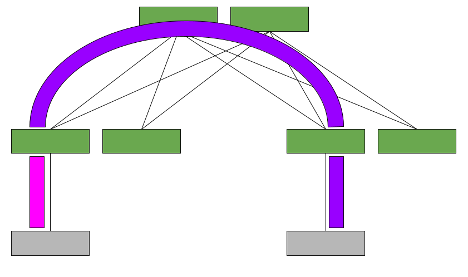
Consider the example from earlier. Host A wants to communicate with Host B, which is located on a different VLAN and a different rack, thus reachable through a different VNI.
With the asymmetric model, all the required source and destination VNIs (for example, orange and green) must be present on each leaf, even if that leaf doesn’t have a host in that VLAN in its rack. This may increase the number of IP/MAC addresses that the leaf must hold, which results in somewhat limited scale. However, in many instances, all VNIs in the network are configured on all leaves anyway to allow VM mobility and to simplify configuration of the whole network. In this case, the asymmetric model is desirable.
While it is not hugely scalable, deployment with the asymmetric model is a simple solution, as no additional VNIs or VLANs must be configured. Additionally, fewer routing hops occur to communicate between VXLANs, which results in lower latency.
Where multitenancy is required, each set of VLANs can also be placed into separate VRFs and routed between the VLANs within a VRF.
The symmetric model routes and bridges on both the ingress and the egress leaves. This results in bidirectional traffic being able to travel on the same VNI, hence the symmetric name.
However, a new specialty transit VNI is used for all routed VXLAN traffic, called the L3VNI. All traffic that must be routed is routed onto the L3VNI, tunneled across the layer 3 infrastructure, routed off the L3VNI to the appropriate VLAN, and ultimately bridged to the destination.
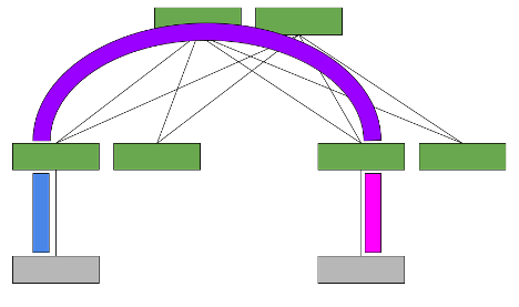
Now consider the scenario with a symmetric model (Figure 2). Host A on VLAN A must communicate with Host B on VLAN B.
With symmetric model, the leaf switches only need to host the VLANs and the corresponding VNIs that are located on its rack, as well as the L3VNI and its associated VLAN. This is because the ingress leaf switch doesn’t need to know the destination VNI.
The ability to host only the local VNIs (plus one extra) helps with scale. However, the configuration is more complex as an extra VXLAN tunnel and VLAN in your network are required. The data plane traffic is also more complex as an extra routing hop occurs and could cause extra latency.
Multitenancy requires one L3VNI per VRF, and all switches participating in that VRF must be configured with the same L3VNI. The L3VNI is used by the egress leaf to identify the VRF in which to route the packet.
The hardest part of choosing an IRB model is knowing the difference between symmetric and asymmetric methods. Now that you know the difference, you can make an informed decision regarding the best option for your network.
Generally, if you configure all VLANs, subnets, or VNIs on all leaves anyway (for mobility or ease of configuration), the asymmetric model is for you. It’s simpler to configure and doesn’t require extra VNIs to troubleshoot. It may even have slightly less latency.
The asymmetric model also works well if your data center can be broken down into Pods with VLANs and subnets contained in a Pod. Each leaf within the Pod is configured with all VLANs and subnets or VNIs in that local Pod. Other Pods and external networks are reachable through EVPN external routes. EVPN external routing with the asymmetric model is supported in Cumulus Linux 3.6 release, using the L3VNI for external routing only.
If your VLANs, subnets, or VNIs are widely dispersed or provisioned on the fly, choose the symmetric model. The symmetric model supports reachability to external networks with Cumulus Linux 3.5.
NVIDIA believes that you own and control your network, not a proprietary vendor, so we provide both solutions and enable you to choose.
 Industry luminaries joined us to introduce the fundamentals of real-time ray tracing, and how current developers such as Autodesk, Dassault, Chaos and ESI have integrated ray traced technologies into their most popular apps.
Engineers, product developers and designers around the world attended GTC to experience the latest NVIDIA solutions that are accelerating interactive rendering and simulation workflows in real time.
We showcased a wide variety of NVIDIA-powered ray tracing technologies and features that provide more realistic visualizations for artists and designers worldwide. Industry luminaries joined us at GTC to introduce the fundamentals of real-time ray tracing and how current developers such as Autodesk, Dassault, Chaos and ESI have integrated ray traced technologies into their most popular applications.
All of these GTC sessions are now available through NVIDIA On-Demand, so learn more about ray tracing and catch up on the latest advancements in professional content creation, from real-time ray traced shadows to real-time denoising.
The developer resources listed below are exclusively available to NVIDIA Developer Program members. Join today for free to get access to the tools and training necessary to build on NVIDIA’s technology platform here.
On-Demand Sessions
Ray Tracing in One Weekend
Pete Shirley gets you started on the fundamentals of ray tracing.
Incorporating Real-Time Ray Tracing in Autodesk’s Next-Generation Viewport System
Learn how Autodesk radically improves the quality and performance of their viewport experience by leveraging DXR and Vulkan Ray Tracing.
Real-Time Ray-Traced Effects for CAD: A Developer Story
Hear from Dassault Systèmes on how real-time ray traced shadows enhances the design review workflow for CATIA CAD users.
From Production Rendering with V-Ray GPU to Real-Time Ray Tracing with Chaos Vantage
Get an exclusive peek on the latest advancements in V-Ray and Chaos Vantage.
Not Just for Games: Applying NVIDIA Real-Time Denoisers in Advanced Immersive Virtual Prototyping
See how ESI group is computing physically correct, high-quality ambient occlusion and soft shadows for the most complex CAD models.
Check out all the ray tracing sessions from GTC, now available for free on NVIDIA On-Demand.
 The NVIDIA NGC catalog is a hub of highly performant software containers, pre-trained models, industry specific SDKs and Helm charts you can simplify and accelerate your end-to-end workflows.
The NVIDIA NGC catalog is a hub of GPU-optimized deep learning, machine learning and HPC applications. With highly performant software containers, pre-trained models, industry specific SDKs and Helm charts you can simplify and accelerate your end-to-end workflows.
The NVIDIA NGC team works closely with our internal and external partners to update the content in the catalog on a regular basis. Below are some of the highlights:
NVIDIA Maxine is a GPU-accelerated SDK with state-of-the-art AI features for developers to build virtual collaboration and content creation solutions, including video conferencing and streaming applications. You can add any of Maxine’s AI effects – Video, Audio, and Augmented Reality – into your existing application or develop a new pipeline from scratch.
Maxine’s Video Effects SDK and Audio Effects SDK are now available through the Maxine collection on the NGC catalog that includes a container for each SDK:
Clara Train v4.0 is now powered by MONAI, a domain-specialized open-source PyTorch framework, accelerating deep learning in Healthcare imaging.
The latest version also expands into Digital Pathology and introduces homomorphic encryption for server side aggregation in federated learning.
The NVIDIA Transfer Learning Toolkit (TLT) is the AI toolkit that abstracts away the AI/DL framework complexity and leverages high quality pre-trained models to enable you to build production quality models faster with only a fraction of data required.
Version 3.0 of TLT is now available for computer vision and conversational AI use cases. Get started today by exploring the TLT collections for:
Our most popular deep learning frameworks for training and inference have also been updated to the latest 21.02 version
 The Game Developer Conference (GDC) is here, and NVIDIA will be showcasing how our latest technologies are driving the future of game development and graphics. Check out our list of sessions now.
The Game Developer Conference (GDC) is here, and NVIDIA will be showcasing how our latest technologies are driving the future of game development and graphics.
From NVIDIA Deep Learning Super Sampling (DLSS) to RTX Global Illumination (RTXGI), our latest tools and technologies are helping game developers create realistic and stunning virtual worlds for gamers. Attendees will also get an exclusive look at how NVIDIA Omniverse, the open platform for virtual collaboration and simulation, is helping developers accelerate production workflows.
And don’t miss our sessions at GDC:
Collaborative Game Development with NVIDIA Omniverse
Get an inside look at all the collaboration tools available in Omniverse. Explore the platform’s ability to connect popular tools and applications, including Epic Games’ Unreal Engine 4, Autodesk Maya and 3ds Max, and Substance by Adobe.
Learn more about the NVIDIA RTX Unreal Engine Branch (NvRTX), and discover technologies such as RTXDI, RTXGI, new denoisers like Relax, ray-traced volumetrics and tools like the BVH viewer. See demonstrations on how complex settings like a jungle or museum can be built with NvRTX, and get a better understanding of how AAA real-time ray tracing visuals are created.
NVIDIA DLSS Overview & Game Integrations
This session will cover the technology that makes DLSS possible. Learn how to integrate DLSS into a new game engine. Graphic programmers, technical artists and technical directors are encouraged to join this session so they can learn more about the engine requirements for DLSS and pick up general DLSS debugging tools.
Game developers can dive into the NvRTX family of branches, and learn how to bring enhanced ray tracing support to Unreal Engine 4. This session will cover several challenges developers can encounter when working to deploy ray tracing in a game environment. Join us and explore how NVIDIA has crafted solutions for these challenges within the context of a curated branch of UE4.
DevTools for Harnessing Ray Tracing in Games
Students, technical artists, programmers and developers can experience ray tracing at interactive framerates with DXR and Vulkan Ray Tracing. Join this session to check out some of the available tools and features that developers can use to take advantage of NVIDIA GPUs and improve the graphics in games.
Enter for a Chance to Win Some Gems

Attendees can win a limited-edition hard copy of Ray Tracing Gems II, the follow up to 2019’s Ray Tracing Gems.
Ray Tracing Gems II brings the community of rendering experts back together to share their knowledge. The book covers everything in ray tracing and rendering, from basic concepts geared toward beginners to full ray tracing deployment in shipping AAA games.
Learn more about the sweepstakes and enter for a chance to win.
Register for GDC today and join us to get the latest on NVIDIA technology in the gaming industry.
Wake up, wake up, wake up, it’s the first of the month. This first of the month is a GFN Thursday celebration. The Steam Summer Sale now has over 700 PC games on sale that are playable on GeForce NOW. And since it’s also the first GFN Thursday of the month, it’s time to check Read article >
The post GFN Thursday Goes Full Steam Ahead: Over 700 Steam Summer Sale Games Streaming on GeForce NOW appeared first on The Official NVIDIA Blog.
![[C[i,j] = Sigma_{r = 1}^{n} A[i,r] cdot B[r,j]]](https://s0.wp.com/latex.php?latex=%5BC%5Bi%2Cj%5D+%3D+%5CSigma_%7Br+%3D+1%7D%5E%7Bn%7D+A%5Bi%2Cr%5D+%5Ccdot+B%5Br%2Cj%5D%5D&bg=ffffff&fg=000&s=0&c=20201002)
![[C[i,j] = textrm{atomicAdd}(C[i,j], A[i, textrm{tid}(i,j)] cdot B[textrm{tid}(i,j), j])]](https://s0.wp.com/latex.php?latex=%5BC%5Bi%2Cj%5D+%3D+%5Ctextrm%7BatomicAdd%7D%28C%5Bi%2Cj%5D%2C+A%5Bi%2C+%5Ctextrm%7Btid%7D%28i%2Cj%29%5D+%5Ccdot+B%5B%5Ctextrm%7Btid%7D%28i%2Cj%29%2C+j%5D%29%5D&bg=ffffff&fg=000&s=0&c=20201002)