To say it with the words of Eamonn Keogh: “Time series is a ubiquitous and increasingly prevalent type of data […]”. Virtually any incrementally measured signal, be it along a time axis or a linearly ordered set, can be treated as time series. Examples include electrocardiograms, temperature or voltage measurements, audio, server logs, but also … Continued
To say it with the words of Eamonn Keogh: “Time series is a ubiquitous and increasingly prevalent type of data […]”. Virtually any incrementally measured signal, be it along a time axis or a linearly ordered set, can be treated as time series. Examples include electrocardiograms, temperature or voltage measurements, audio, server logs, but also heavy-weight data such as video and time-resolved MRI volumes. Hence, the efficient yet exact processing of the ever-increasing amount of time series data is crucial for every data scientist.
In this blog, we introduce rapidAligner – a CUDA-accelerated library to align a short time series snippet (query) in an exceedingly long stream of time series (subject) using the following three popular lock-step measures for the local alignment of uniformly sampled time series:
- Rolling Euclidean distance (sdist)
- Rolling mean-adjusted Euclidean distance (mdist)
- Rolling mean and amplitude-adjusted Euclidean distance (zdist)
The rapidAligner library is free software that can be integrated with a broad variety of popular data science and machine learning frameworks such as NumPy, CuPy, RAPIDS, Numba, and Pytorch. The source code is publicly available under NVIDIA rapidAligner.
The rest of the article is structured as follows: Section one provides a brief introduction on popular lock-step measures and (local) normalization techniques. Section two demonstrates the usage of the rapidAligner library. Section 3 concludes this blog post.
A brief introduction to time series data mining
Time series are sequences of pairs (t[i], x[i]) where the real-valued time stamps t[i] are linearly ordered and their corresponding values x[i] are quantities measured at time t[i]. If all timestamps are equally spaced, i.e., t[i+1]-t[i] = const for all i, then you can neglect time and call the sequence of measurements x[i] a uniformly sampled time series. In the following, we will simply refer to uniformly sampled time series with real-valued scalars x[i] as time series without fancy attributes.
Assume you want to compare two time series Q=(q[0], q[1], …, q[m-1]) and S=(s[0], s[1], …, s[m-1]) of same length |Q|=|S|=m. An obvious way would be to interpret Q and S as m-dimensional vectors and compute the Lp norm of their difference.
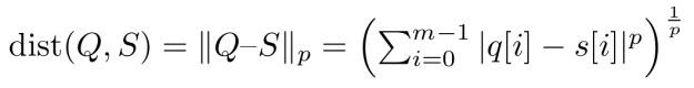
Popular choices for the parameter p are p=2 for so-called Euclidean distance and p=1 for so-called Manhattan or taxicab distance (see Figure 1). In this blog post, we address similarity measures that compare residues q[i]-s[i] using a one-to-one assignment i->i of indices – so-called lock-step measures. In a future post, we will discuss CUDA-accelerated measures using dynamic assignments of indices such as q[i]-s[j], also known as the class of elastic measures.
However, when aligning a short query Q of length |Q|=m in a long stream S of length |S|=n, i.e., 0
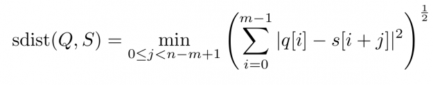
For each alignment position j you have to sum over m contributions. As a result, the asymptotic worst-case complexity to compute all lock-step alignments is proportional to the product of the time series lengths m and n — O((n-m+1) * m) to be precise. This number can be huge even for moderately sized queries and streams which may render large scale time series alignment computationally intractable when performed in a naïve way. In Section 3 we will discuss for the special case p=2 how to implement a CUDA-accelerated scheme which runs in blazingly fast log-linear time.
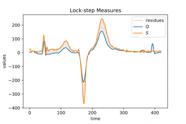
When looking at larger portion of an ECG stream (see Figure 2) you may observe a temporal drift in the average signal value, also known as baseline wandering. This artifact often occurs in continuously measured time series and may be caused by a broad variety of external factors such as change of skin conductivity due to sweat in ECGs, body movement affecting the electrodes in ECGs, drift of electric resistance and thus voltage due to temperature variation in power supplies, temperature drift when recording environmental quantities, seasonal effects such as Christmas, or the temporal drift of stock prices amidst a global pandemic.
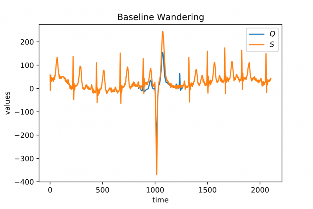
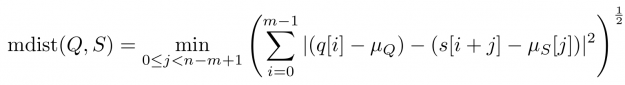
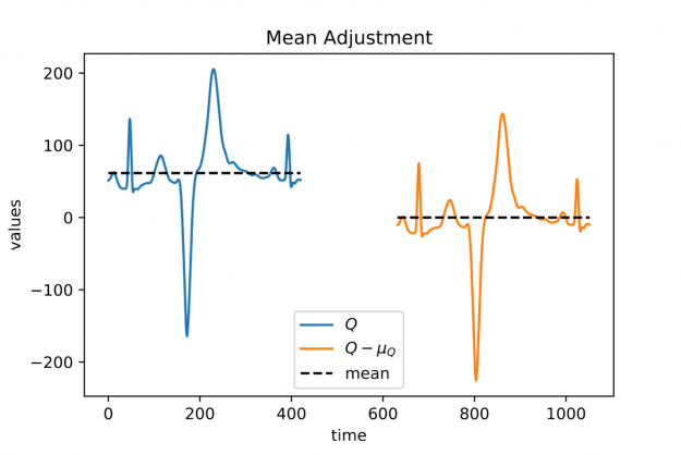
Baseline wandering is problematic when mining a stream for similar shapes – two similar shapes with different offsets on the measurement axis may have a larger distance than two dissimilar ones with similar offsets. A surprisingly simple and effective countermeasure is to introduce a normalization procedure for the query and candidate sequences. As an example, you could compute the mean value of the query muQ and for each of the n-m+1 candidate sequences muS[j] to remove the offset in the corresponding window (see Figure 3). In the following, we will call locally mean-adjusted rolling Euclidean distance mdist:
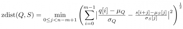
A closer look at Figure 1 and Figure 2 further reveals a temporal variation in amplitudes. The range of values in the blue query is significantly smaller than the amplitude of the orange candidate sequence in Figure 1. Temporal drift in the scale might lead to meaningless matches when mining shapes. A straightforward solution is to normalize the scale by dividing the values by the standard deviation of the query sigmaQ and alignment candidates sigmaS[j], respectively. The proposed mean and amplitude adjustment is called z-normalization referring to z-scores of normal random variables with vanishing mean and unit variance (see Figure 4). The corresponding rolling measure shall be called zdist:
The library rapidAligner supports the CUDA-accelerated computation of the three aforementioned rolling measures sdist, mdist, and zdist in a massively parallel fashion. In the next section, you will see its simple usage from within JupyterLab.
rapidAligner in action
Let’s start crunching numbers. In this section, you will align a single heartbeat in a 22 hour ECG stream using the three discussed measures sdist, mdist, and zdist. The data set is part of the experiments listed on the website of the award-winning UCR-Suite. After cloning the rapidAligner repository you immediately import the rapidAligner library alongside with CuPY, NumPy, and Matplotlib for later validation and visualization.
In the next step, you load the ECG data. The length of the query is rather short with 421 entries, yet the stream exhibits roughly 20 million time ticks. A first inspection of the full query (blue) and the initial 1000 values of the stream (orange) reveals temporal drift in both offsets and amplitudes.
In the following, you align the query in the stream using the sdist measure computing all 20,140,000-421+1 distance scores a subsequent argmin-reduction to determine the best alignment position. For our experiments we choose a single A100 GPU in a DGX A100 server. Note that if you are only interested in the best match one could further accelerate the already rapid computation by employing a lower-bound cascade as demonstrated here. In contrast, rapidAligner’s sdist call returns alignment scores for all positions to allow for later processing such as computing a non-overlapping partition of ranked matches. We further repeat the alignment a few times for robust runtime measurement. Both compute modes “fft” and “naive” are blazingly fast and return indistinguishable results:
- “naive”: all n-m+1 alignment candidates are (optionally) normalized and compared individually with a minimal memory footprint but O(n*m) asymptotic computational complexity. This mode is still reasonably fast using warp-aggregated statistics and accumulation schemes.
- “fft”: If m > log_2(n), we can exploit the Convolution Theorem to accelerate the computation significantly resulting in O(n * log n) runtime but a higher memory footprint. This compute mode is fully independent of the query’s length and thus advisable for large input. The higher memory usage is mainly caused by computationally fast but out-of-place primitives such as CUDA-accelerated Fast Fourier Transforms and Prefix Scans.
Both the query and stream (subject) are stored as plain NumPy arrays in double precision on the CPU. As a result, the measured runtimes include costly memory transfers between the CPU and GPU. rapidAligner allows for seamless interoperability with all CUDA array interface compliant frameworks such as PyTorch, CuPy, Numba, RAPIDS, and Jax. Hence, you can further reduce the runtime when caching the data in fast GPU RAM to avoid unnecessary memory movement between CPU and GPU. Now, it becomes even more obvious that the Fourier based mode outperforms the naïve one even on short queries
That corresponds to a whopping 2.5 billion full alignments per second on a single GPU. In the following, we report runtimes exclusively using input data residing on the GPU. The match produced by sdist is already a good one but let us check if mean-adjustment improves the result:
As expected, mean adjustment returns a better match since now candidates are considered with a non-vanishing relative offset along the measurement axis. The execution times remain low with 10 ms for 20 million alignment positions. That corresponds to 2 billion full alignments per second. You could still improve the amplitude mismatch using zdist:
Et voilà, z-normalized rolling Euclidean distance reveals a doppelgänger in the database which is almost indistinguishable from the query. Performance remains high in more than 1.6 billion alignments per second. A stunning property of the Fourier mode is that the runtime is effectively independent of the query length, i.e., the runtime is constant for fixed stream length and varying query size. This becomes handy when aligning extra-ordinarily long queries.
Conclusion
Finding shapes in long streams of time series data is a computationally demanding task frequently occurring as a standalone routine or embedded as a subroutine in high-level algorithms, e.g., for the detection of anomalies. Hence, massively parallel accelerators with their unprecedented memory bandwidth such as the NVIDIA A100 GPU are ideally suited to address this challenge. rapidAligner is lightweight library processing billions of alignments per second while supporting common normalization modes for the candidate sequences. You can further employ highly optimized FFT routines cuFFT and prefix scans CUB from the CUDA-X software stack to provide an alignment mode that is independent from the query length. The source code and notebooks are publicly available under NVIDIA rapidAligner
Happy time series mining!


 Today, NVIDIA is announcing the availability of cuTENSOR version 1.3.0. This software can be downloaded now free for members of the NVIDIA Developer Program.
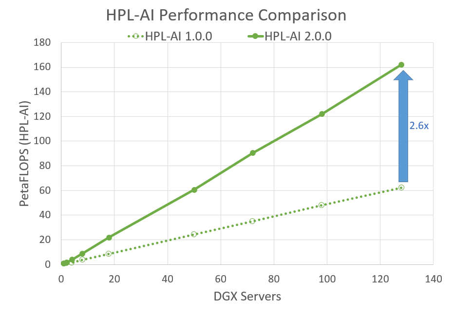
 NVIDIA announced its latest update to the HPL-AI Benchmark version 2.0.0, which will reside in the HPC-Benchmarks container version 21.4.