import tensorflow as tf
physical_devices = tf.config.experimental.list_physical_devices(‘GPU’)
if len(physical_devices) > 0:
tf.config.experimental.set_memory_growth(physical_devices[0], True)
from absl import app, flags, logging
from absl.flags import FLAGS
import core.utils as utils
from core.yolov4 import filter_boxes
from tensorflow.python.saved_model import tag_constants
from PIL import Image
import cv2
import numpy as np
from tensorflow.compat.v1 import ConfigProto
from tensorflow.compat.v1 import InteractiveSession
flags.DEFINE_string(‘framework’, ‘tf’, ‘(tf, tflite, trt’)
flags.DEFINE_string(‘weights’, ‘./checkpoints/yolov4-416’,
‘path to weights file’)
flags.DEFINE_integer(‘size’, 416, ‘resize images to’)
flags.DEFINE_boolean(‘tiny’, False, ‘yolo or yolo-tiny’)
flags.DEFINE_string(‘model’, ‘yolov4’, ‘yolov3 or yolov4’)
flags.DEFINE_string(‘image’, ‘./data/kite.jpg’, ‘path to input image’)
flags.DEFINE_string(‘output’, ‘result.png’, ‘path to output image’)
flags.DEFINE_float(‘iou’, 0.45, ‘iou threshold’)
flags.DEFINE_float(‘score’, 0.25, ‘score threshold’)
def main(_argv):
config = ConfigProto()
config.gpu_options.allow_growth = True
session = InteractiveSession(config=config)
STRIDES, ANCHORS, NUM_CLASS, XYSCALE = utils.load_config(FLAGS)
input_size = FLAGS.size
image_path = FLAGS.image
original_image = cv2.imread(image_path)
original_image = cv2.cvtColor(original_image, cv2.COLOR_BGR2RGB)
# image_data = utils.image_preprocess(np.copy(original_image), [input_size, input_size])
image_data = cv2.resize(original_image, (input_size, input_size))
image_data = image_data / 255.
# image_data = image_data[np.newaxis, …].astype(np.float32)
images_data = []
for i in range(1):
images_data.append(image_data)
images_data = np.asarray(images_data).astype(np.float32)
if FLAGS.framework == ‘tflite’:
interpreter = tf.lite.Interpreter(model_path=FLAGS.weights)
interpreter.allocate_tensors()
input_details = interpreter.get_input_details()
output_details = interpreter.get_output_details()
print(input_details)
print(output_details)
interpreter.set_tensor(input_details[0][‘index’], images_data)
interpreter.invoke()
pred = [interpreter.get_tensor(output_details[i][‘index’]) for i in range(len(output_details))]
if FLAGS.model == ‘yolov3’ and FLAGS.tiny == True:
boxes, pred_conf = filter_boxes(pred[1], pred[0], score_threshold=0.25, input_shape=tf.constant([input_size, input_size]))
else:
boxes, pred_conf = filter_boxes(pred[0], pred[1], score_threshold=0.25, input_shape=tf.constant([input_size, input_size]))
else:
saved_model_loaded = tf.saved_model.load(FLAGS.weights, tags=[tag_constants.SERVING])
infer = saved_model_loaded.signatures[‘serving_default’]
batch_data = tf.constant(images_data)
pred_bbox = infer(batch_data)
for key, value in pred_bbox.items():
boxes = value[:, :, 0:4]
pred_conf = value[:, :, 4:]
boxes, scores, classes, valid_detections = tf.image.combined_non_max_suppression(
boxes=tf.reshape(boxes, (tf.shape(boxes)[0], -1, 1, 4)),
scores=tf.reshape(
pred_conf, (tf.shape(pred_conf)[0], -1, tf.shape(pred_conf)[-1])),
max_output_size_per_class=50,
max_total_size=50,
iou_threshold=FLAGS.iou,
score_threshold=FLAGS.score
)
pred_bbox = [boxes.numpy(), scores.numpy(), classes.numpy(), valid_detections.numpy()]
image = utils.draw_bbox(original_image, pred_bbox)
image = Image.fromarray(image.astype(np.uint8))
image.show()
image = cv2.cvtColor(np.array(image), cv2.COLOR_BGR2RGB)
cv2.imwrite(FLAGS.output, image)
if __name__ == ‘__main__’:
try:
app.run(main)
except SystemExit:
pass
PLZ HELP ME CROP THE BOUNDING BOX IN ORDER TO PERFORM A TESSERACT TO READ WHAT IS INSIDE THE BOUNDING BOX (DIGITS) .This is my work but it doesn’t crop
import tensorflow as tf
physical_devices = tf.config.experimental.list_physical_devices(‘GPU’)
if len(physical_devices) > 0:
tf.config.experimental.set_memory_growth(physical_devices[0], True)
from absl import app, flags, logging
from absl.flags import FLAGS
import core.utils as utils
from core.yolov4 import filter_boxes
from tensorflow.python.saved_model import tag_constants
from PIL import Image
import cv2
import numpy as np
import os
from tensorflow.compat.v1 import ConfigProto
from tensorflow.compat.v1 import InteractiveSession
flags.DEFINE_string(‘framework’, ‘tf’, ‘(tf, tflite, trt’)
flags.DEFINE_string(‘weights’, ‘./checkpoints/yolov4-416’,
‘path to weights file’)
flags.DEFINE_integer(‘size’, 416, ‘resize images to’)
flags.DEFINE_boolean(‘tiny’, False, ‘yolo or yolo-tiny’)
flags.DEFINE_string(‘model’, ‘yolov4’, ‘yolov3 or yolov4’)
flags.DEFINE_string(‘image’, ‘./data/kite.jpg’, ‘path to input image’)
flags.DEFINE_string(‘output’, ‘result.png’, ‘path to output image’)
flags.DEFINE_float(‘iou’, 0.45, ‘iou threshold’)
flags.DEFINE_float(‘score’, 0.25, ‘score threshold’)
flags.DEFINE_boolean(‘crop’, False, ‘crop detections from images’)
def crop_objects (img, data, path){
boxes, scores = data
class_name = “Compteur”
# get box coords
xmin, ymin, xmax, ymax = boxes[i]
# crop detection from image (take an additional 5 pixels around all edges)
cropped_img = img[int(ymin)-5:int(ymax)+5, int(xmin)-5:int(xmax)+5]
# construct image name and join it to path for saving crop properly
img_name = class_name +’.png’
img_path = os.path.join(path, img_name )
# save image
cv2.imwrite(img_path, cropped_img)
}
# helper function to convert bounding boxes from normalized ymin, xmin, ymax, xmax —> xmin, ymin, xmax, ymax
def format_boxes(bboxes, image_height, image_width):
for box in bboxes:
ymin = int(box[0] * image_height)
xmin = int(box[1] * image_width)
ymax = int(box[2] * image_height)
xmax = int(box[3] * image_width)
box[0], box[1], box[2], box[3] = xmin, ymin, xmax, ymax
return bboxes
def draw_bbox(image, bboxes, info = False, counted_classes = None, show_label=True, allowed_classes=list(read_class_names(cfg.YOLO.CLASSES).values()), read_plate = False):
classes = read_class_names(cfg.YOLO.CLASSES)
num_classes = len(classes)
image_h, image_w, _ = image.shape
hsv_tuples = [(1.0 * x / num_classes, 1., 1.) for x in range(num_classes)]
colors = list(map(lambda x: colorsys.hsv_to_rgb(*x), hsv_tuples))
colors = list(map(lambda x: (int(x[0] * 255), int(x[1] * 255), int(x[2] * 255)), colors))
random.seed(0)
random.shuffle(colors)
random.seed(None)
out_boxes, out_scores, out_classes, num_boxes = bboxes
for i in range(num_boxes):
if int(out_classes[i]) < 0 or int(out_classes[i]) > num_classes: continue
coor = out_boxes[i]
fontScale = 0.5
score = out_scores[i]
class_ind = int(out_classes[i])
class_name = classes[class_ind]
if class_name not in allowed_classes:
continue
else:
if read_plate:
height_ratio = int(image_h / 25)
plate_number = recognize_plate(image, coor)
if plate_number != None:
cv2.putText(image, plate_number, (int(coor[0]), int(coor[1]-height_ratio)),
cv2.FONT_HERSHEY_SIMPLEX, 1.25, (255,255,0), 2)
bbox_color = colors[class_ind]
bbox_thick = int(0.6 * (image_h + image_w) / 600)
c1, c2 = (coor[0], coor[1]), (coor[2], coor[3])
cv2.rectangle(image, c1, c2, bbox_color, bbox_thick)
if info:
print(“Object found: {}, Confidence: {:.2f}, BBox Coords (xmin, ymin, xmax, ymax): {}, {}, {}, {} “.format(class_name, score, coor[0], coor[1], coor[2], coor[3]))
if show_label:
bbox_mess = ‘%s: %.2f’ % (class_name, score)
t_size = cv2.getTextSize(bbox_mess, 0, fontScale, thickness=bbox_thick // 2)[0]
c3 = (c1[0] + t_size[0], c1[1] – t_size[1] – 3)
cv2.rectangle(image, c1, (np.float32(c3[0]), np.float32(c3[1])), bbox_color, -1) #filled
cv2.putText(image, bbox_mess, (c1[0], np.float32(c1[1] – 2)), cv2.FONT_HERSHEY_SIMPLEX,
fontScale, (0, 0, 0), bbox_thick // 2, lineType=cv2.LINE_AA)
if counted_classes != None:
height_ratio = int(image_h / 25)
offset = 15
for key, value in counted_classes.items():
cv2.putText(image, “{}s detected: {}”.format(key, value), (5, offset),
cv2.FONT_HERSHEY_COMPLEX_SMALL, 1, (0, 255, 0), 2)
offset += height_ratio
return image
def main(_argv):
config = ConfigProto()
config.gpu_options.allow_growth = True
session = InteractiveSession(config=config)
STRIDES, ANCHORS, NUM_CLASS, XYSCALE = utils.load_config(FLAGS)
input_size = FLAGS.size
image_path = FLAGS.image
original_image = cv2.imread(image_path)
original_image = cv2.cvtColor(original_image, cv2.COLOR_BGR2RGB)
# image_data = utils.image_preprocess(np.copy(original_image), [input_size, input_size])
image_data = cv2.resize(original_image, (input_size, input_size))
image_data = image_data / 255.
# image_data = image_data[np.newaxis, …].astype(np.float32)
images_data = []
for i in range(1):
images_data.append(image_data)
images_data = np.asarray(images_data).astype(np.float32)
if FLAGS.framework == ‘tflite’:
interpreter = tf.lite.Interpreter(model_path=FLAGS.weights)
interpreter.allocate_tensors()
input_details = interpreter.get_input_details()
output_details = interpreter.get_output_details()
print(input_details)
print(output_details)
interpreter.set_tensor(input_details[0][‘index’], images_data)
interpreter.invoke()
pred = [interpreter.get_tensor(output_details[i][‘index’]) for i in range(len(output_details))]
if FLAGS.model == ‘yolov3’ and FLAGS.tiny == True:
boxes, pred_conf = filter_boxes(pred[1], pred[0], score_threshold=0.25, input_shape=tf.constant([input_size, input_size]))
else:
boxes, pred_conf = filter_boxes(pred[0], pred[1], score_threshold=0.25, input_shape=tf.constant([input_size, input_size]))
else:
saved_model_loaded = tf.saved_model.load(FLAGS.weights, tags=[tag_constants.SERVING])
infer = saved_model_loaded.signatures[‘serving_default’]
batch_data = tf.constant(images_data)
pred_bbox = infer(batch_data)
for key, value in pred_bbox.items():
boxes = value[:, :, 0:4]
pred_conf = value[:, :, 4:]
boxes, scores, classes, valid_detections = tf.image.combined_non_max_suppression(
boxes=tf.reshape(boxes, (tf.shape(boxes)[0], -1, 1, 4)),
scores=tf.reshape(
pred_conf, (tf.shape(pred_conf)[0], -1, tf.shape(pred_conf)[-1])),
max_output_size_per_class=50,
max_total_size=50,
iou_threshold=FLAGS.iou,
score_threshold=FLAGS.score
)
# format bounding boxes from normalized ymin, xmin, ymax, xmax —> xmin, ymin, xmax, ymax
original_h, original_w, _ = original_image.shape
bboxes = format_boxes(boxes.numpy()[0], original_h, original_w)
# hold all detection data in one variable
pred_bbox = [bboxes, scores.numpy()[0], classes.numpy()[0], valid_detections.numpy()[0]]
image = utils.draw_bbox(original_image, pred_bbox)
# image = utils.draw_bbox(image_data*255, pred_bbox)
image = Image.fromarray(image.astype(np.uint8))
image.show()
image = cv2.cvtColor(np.array(image), cv2.COLOR_BGR2RGB)
cv2.imwrite(FLAGS.output, image)
# if crop flag is enabled, crop each detection and save it as new image
if FLAGS.crop:
crop_path = os.path.join(os.getcwd(), ‘detections’, ‘crop’, image_name)
try:
os.mkdir(crop_path)
except FileExistsError:
pass
crop_objects(cv2.cvtColor(original_image, cv2.COLOR_BGR2RGB), pred_bbox, crop_path)
if __name__ == ‘__main__’:
try:
app.run(main)
except SystemExit:
pass

 Google Cloud and NVIDIA collaborated to make MLOps simple, powerful, and cost-effective by bringing together the solution elements to build, serve and dynamically scale your end-to-end ML pipelines with the right-sized GPU acceleration in one place.


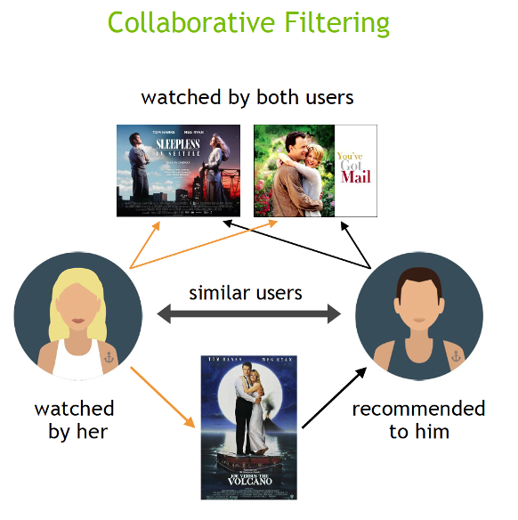
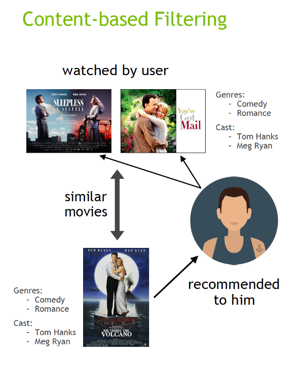
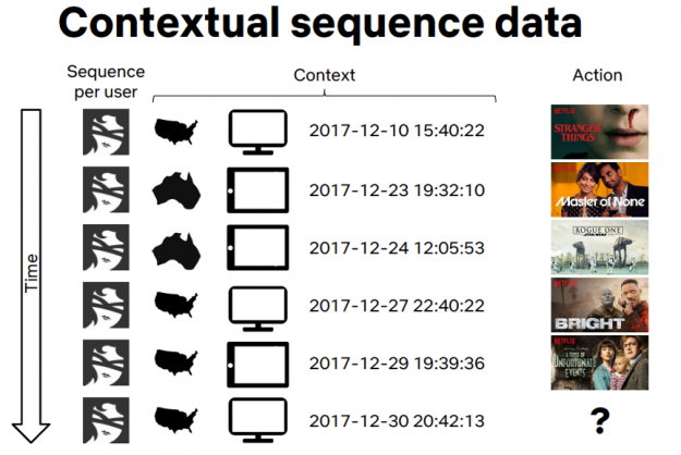
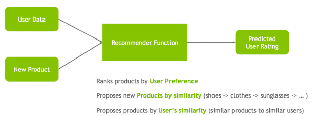
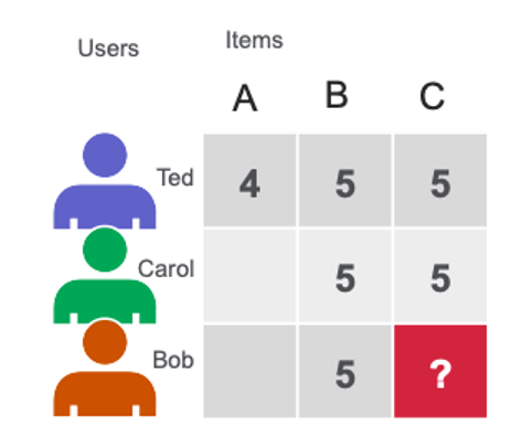
 Recommender systems (RecSys) have become a key component in many online services, such as e-commerce, social media, news service, or online video streaming. However with their growth in importance, the growth in scale of industry datasets, and more sophisticated models, the bar has been raised for computational resources required for recommendation systems. After NVIDIA introduced Merlin …
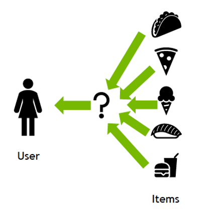

 A recent National Poetry Month feature in The Washington Post presented AI-generated artwork alongside five original poems reflecting on seasons of the past year.
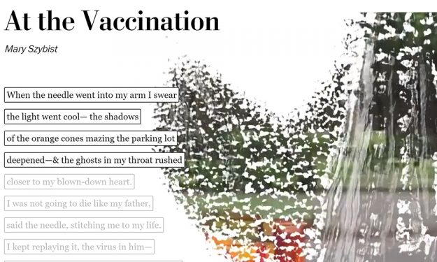
 NVIDIA announced the availability of cuSPARSELt version 0.1.0. This software can be downloaded now free for members of the NVIDIA Developer Program.
 cdot op(B) + beta op(C)")
") and
and ") refer to in-place operations such as transpose/non-transpose.
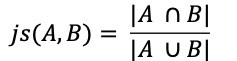
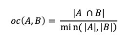
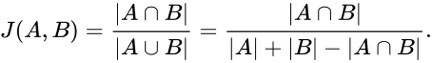
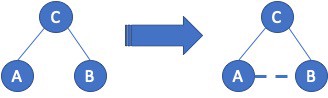
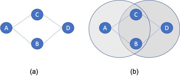
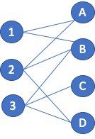
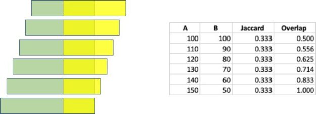
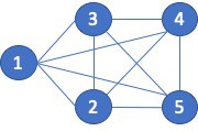
refer to in-place operations such as transpose/non-transpose. There is a wide range of graph applications and algorithms that I hope to discuss through this series of blog posts, all with a bias toward what is in RAPIDS cuGraph. I am assuming that the reader has a basic understanding of graph theory and graph analytics. If there is interest in a graph analytic …