Thousands of U.S. traffic lights may soon be getting the green light on AI for safer streets. That’s because startup CVEDIA has designed better and faster vehicle and pedestrian detections to improve traffic flow and pedestrian safety for Cubic Transportation Systems. These new AI capabilities will be integrated into Cubic’s GRIDSMART Solution, a single-camera intersection Read article >
In AI and computer vision, data acquisition is costly and time-consuming and human-based labeling can be error-prone. The accuracy of the models is also affected by insufficient and poorly balanced data and the prolonged time required to improve the deep learning models. It always requires the reacquisition of data in the real world. The collection, … Continued
In AI and computer vision, data acquisition is costly and time-consuming and human-based labeling can be error-prone. The accuracy of the models is also affected by insufficient and poorly balanced data and the prolonged time required to improve the deep learning models. It always requires the reacquisition of data in the real world.
The collection, preparation of data, and development of accurate and reliable software solutions based on AI training is an extremely laborious process. The required investment costs offset the expected benefits of deploying the system.
One way to bridge the data gap and accelerate model training is by using synthetic data instead of real data for training. SKY ENGINE provides an AI platform to move deep learning to virtual reality. It is possible to generate synthetic data using simulations where the synthetic images come with the annotation that can be used directly in training AI models.
Synthetic data can now be directly exported to run on the NVIDIA Transfer Learning Toolkit (TLT), an AI training toolkit that simplifies training by abstracting away the AI/DL framework complexity. This enables you to build production-quality models faster without needing any AI expertise. With the SKY ENGINE AI platform and TLT, you can quickly iterate and build AI.
In this post, you learn how you can harness the power of synthetic data by taking preannotated synthetic data and training it on TLT. I demonstrate a simple inspection use case to identify antennas on a telco tower using segmentation.
About the SKY ENGINE AI approach
SKY ENGINE introduces a full-stack AI platform for deep learning in virtual reality, which is the next-generation active learning AI system for image and video analysis applications. The SKY ENGINE AI platform can generate data using a proprietary, dedicated simulation system where images come already annotated and ready for deep learning.
The output data stream can include any of the following:
Rendered images or other simulated sensor data in selected modalities
Object bounding boxes
3D bounding boxes
Semantic masks
2D or 3D skeletons
Depth maps
Normal vector maps
SKY ENGINE AI also includes advanced domain adaptation algorithms that can understand the characteristics of real data examples. They assure the high-quality performance of any trained AI model during the inference.
Figure 1. SKY ENGINE AI platform user interface preview.
The SKY ENGINE simulation system enables physics-driven sensor simulations (cameras, thermal vision, IR, lidars, radars, and more) and sensor data fusion. It is tightly coupled with a deep learning pipeline to ensure evolution. During training, SKY ENGINE AI can spot ambiguous situations that deteriorate the accuracy of the AI model. It obtains more imagery data to reflect those problematic situations that the deep learning accuracy could instantaneously improve. SKY ENGINE AI learns more with every performed experiment.
SKY ENGINE AI delivers a garden of deep neural networks fully implemented, tested, and optimized. Provided models are dedicated to popular computer vision tasks like object detection and semantic segmentation. They can also serve as more sophisticated topologies designed and implemented for 3D position and pose estimation, 3D geometry reasoning, or representation learning.
SKY ENGINE AI also includes advanced domain adaptation algorithms that can understand the characteristics of real data examples and assure the performance of trained model inference. SKY ENGINE AI does not require sophisticated rendering and imaging knowledge, so the entry barrier is very low. It has a Python API, including a large number of helpers to quickly build and configure the environment.
Neural network optimization
The SKY ENGINE AI platform can generate the datasets and enable the training of deep learning models that can use input data originating from any source. The input stream for AI models training in NVIDIA TLT and AI-driven inference can effectively include low-quality images obtained using smartphones, data from CCTV cameras, or cameras mounted on drones.
You can deploy analytical modules for telecommunication network performance optimization on the cloud, including data storage and multi-GPU scaling. The majority of software projects driven by machine learning in this space are unable to reach the final stage of solution deployment. This could be because of the high dependence of machine learning capabilities on the quality of the input data. The development of AI models with deep training on synthetic data, offered by SKY ENGINE, is a solution with predictable project development and guaranteed deployment in several industrial business processes.
Telecommunication equipment detection and classification
One of the common computer vision tasks is the localization and classification of the equipment of interest. In this post, I present the process of neural network optimization for bounding box localization of antenna instances on a telecommunication tower using the NVIDIA TLT environment with MaskRCNN. You use the synthetic data from SKY ENGINE AI to train the MaskRCNN model. The high-level workflow is as follows:
Generate synthetic data with annotations.
Convert the data format to COCO as required by NVIDIA TLT MaskRCNN model.
Configure the NGC environment and data preprocessing.
Train and evaluate the MaskRCNN model on synthetic data.
Perform inference using the trained AI model on synthetic and real telco towers.
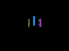
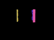
Given the real samples of a telco tower, I used the SE Rendering Engine to create an annotated synthetic dataset.
Figure 2. Synthetic images include automatically applied labels generated in the SKY ENGINE AI platform. (left) Synthetic images; (right) Semantic masks
To launch automatic generation of labeled data using SKY ENGINE AI and to prepare the data source object, you must define basic tools like empty renderer context, as well as paths where the assets for the synthetic scene are located.
In this rendering scenario, I randomized the following:
The number of antennas on a given telecommunication tower
The direction of the light
The positions of the camera
The camera’s horizontal field of view
A background map
There can be many projects in which the samples returned by SKY ENGINE are not shuffled enough. One example would be when your rendering process follows the camera trajectory. For this reason, I recommend extra shuffling of the data before dividing it into train and test sets.
After generating the images, convert them to COCO format using the data export module of SKY ENGINE. This is required by the NVIDIA TLT framework. After you prepare the configuration file according to the documentation, you can run the training for the TLT pretrained Mask RCNN model with the TensorFlow backend:
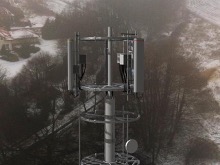
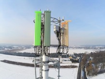
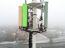
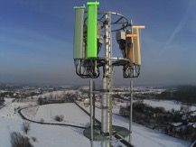
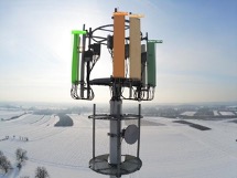
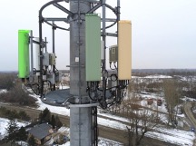
Figure 3 shows some results of telecommunication antenna detection.
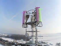
Figure 3. Application of trained AI models on real images.
Summary
In this post, I demonstrated how you can reduce your data collection and annotation effort by using the synthetic data from SKY ENGINE and training and optimizing it with NVIDIA TLT. I presented a single SKY ENGINE AI use case for telecommunication industry. However, this platform unlocks the universe of further potential applications delivering several advanced functionalities:
Automated dataset balancing (active learning)
Domain adaptation
Pretrained deep learning models for 3D reasoning
Simulations of sensors and training of deep learning models for sensor fusion
For more information, see the SKY ENGINE AI solution on GitHub. For more computer vision use cases developed in the SKY ENGINE AI Platform, see the following videos:
The long, cumbersome slog of data procurement has been slowing down innovation in AI, especially in computer vision, which relies on labeled images and video for training. But now you can jumpstart your machine learning process by quickly generating synthetic data using AI.Reverie. With the AI.Reverie synthetic data platform, you can create the exact training … Continued
The long, cumbersome slog of data procurement has been slowing down innovation in AI, especially in computer vision, which relies on labeled images and video for training. But now you can jumpstart your machine learning process by quickly generating synthetic data using AI.Reverie.
With the AI.Reverie synthetic data platform, you can create the exact training data that you need in a fraction of the time it would take to find and label the right real photography. In AI.Reverie’s photorealistic 3D environments, you can generate data for all possible scenarios, including hard to reach places, unusual environmental conditions, and rare or unique events.
Training data generation includes labels. Choose the needed types, such as 2D or 3D bounding boxes, depth masks, and so on. After you test your model, you can return to the platform to quickly generate additional data to improve accuracy. Test and repeat in quick, iterative cycles.
We wanted to test performance of AI.Reverie synthetic data in NVIDIA Transfer Learning Toolkit 3.0. Originally, we set out to replicate the results in the research paper RarePlanes: Synthetic Data Takes Flight, which used synthetic imagery to create object detection models. We discovered new tools in TLT that made it possible to create more lightweight models that were as accurate as, but much faster than, those featured in the original paper.
In this post, we show you how we used the TLT quantized-aware training and model pruning to accomplish this, and how to replicate the results yourself. We show you how to create an airplane detector, but you should be able to fine-tune the model for various satellite detection scenarios of your own.
Figure 1. A synthetic image featuring annotations that denote aircraft type, wing shape, and other distinguishing features.
Access the satellite detection model
To replicate these results, you can clone the GitHub repository and follow along with the included Jupyter notebook.
Generate synthetic data using the AI.Reverie platform and use it with NVIDIA TLT.
Train highly accurate models using synthetic data.
Optimize a model for inference using the TLT.
Prerequisites
We tested the code with Python 3.8.8, using Anaconda 4.9.2 to manage dependencies and the virtual environment. The code may work with different versions of Python and other virtual environment solutions, but we haven’t tested those configurations. We used Ubuntu 18.04.5 LTS and NVIDIA driver 460.32.03 and CUDA Version 11.2. TLT requires driver 455.xx or later.
Set up NGC to be able to download NVIDIA Docker containers. Follow steps 4 and 5 in the TLT User Guide. For more information about the NGC CLI tool, see CLI Install.
Have available at least 250 GB hard disk space to store dataset and model weights.
For this tutorial, you need only download a subset of the data. The following code example is meant to be executed from within the Jupyter notebook. First, create the folders:
TLT uses the KITTI format for object detection model training. RarePlanes is in the COCO format, so you must run a conversion script from within the Jupyter notebook. This converts the real train/test and synthetic train/test datasets.
%run convert_coco_to_kitti.py
There should now be a folder for each dataset split inside of data/kitti that contains the KITTI formatted annotation text files and symlinks to the original images.
Setting up TLT mounts
The notebook has a script to generate a ~/.tlt_mounts.json file. For more information about the various settings, see Running the launcher.
You must turn the KITTI labels into the TFRecord format used by TLT. The convert_split function in the notebook helps you bulk convert all the datasets:
 def convert_split(name):
     !tlt detectnet_v2 dataset_convert --gpu_index 0
         -d /workspace/tlt-experiments/specs/detectnet_v2_tfrecords_{name}.txt
         -o /workspace/tlt-experiments/data/tfrecords/{name}/{name}
 You can then run the conversions:
 convert_split('kitti_real_train')
 convert_split('kitti_real_test')
 convert_split('kitti_synthetic_train')
 convert_split('kitti_synthetic_test')
Download the ResNet18 convolutional backbone
Using your NGC account and command-line tool, you can now download the model:
Download the ResNet18 convolutional backbone
Using your NGC account and command-line tool, you can now download the model:
!ngc registry model download-version nvidia/tlt_pretrained_detectnet_v2:resnet18
 Validation cost: 0.001133
 Mean average_precision (in %): 94.2563

 class name      average precision (in %)
 ------------  --------------------------
 aircraft                         94.2563

 Median Inference Time: 0.003877
 2021-04-06 05:47:00,323 [INFO] __main__: Evaluation complete.
 Time taken to run __main__:main: 0:00:27.031500.
 2021-04-06 05:47:02,466 [INFO] tlt.components.docker_handler.docker_handler: Stopping container.
You then use this function to replace the checkpoint in your template spec with the best performing model from the synthetic-only training.
 with open('./specs/detectnet_v2_train_resnet18_kitti_synth_finetune_10.txt', 'r') as f_in:
     with open('./specs/detectnet_v2_train_resnet18_kitti_synth_finetune_10_replaced.txt', 'w') as f_out:
         out = f_in.read().replace('REPLACE', best_checkpoint)
         f_out.write(out)
You can now begin a TLT training. Start your fine-tuning with the best-performing epoch of the model trained on synthetic data alone, in the previous section.
After training has completed, you should see a best epoch of between 91-93% mAP50, which gets you close to the real-only model performance with only 10% of the real data.
In the notebook, there’s a command to evaluate the best performing model checkpoint on the test set:
You should see something like the following output:
2021-04-06 18:05:28,342 [INFO] iva.detectnet_v2.evaluation.evaluation: step 330 / 339, 0.05s/step
Matching predictions to ground truth, class 1/1.: 100%|█| 14719/14719 [00:00
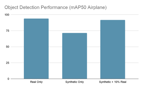
Figure 2. Training on synthetic + 10% real data nearly matches the results of training on 100% of the real data.
Data enhancement is fine-tuning a model training on AI.Reverie’s synthetic data with just 10% of the original, real dataset. As you can see, this technique produces a model as accurate as one trained on real data alone. That represents roughly 90% cost savings on real, labeled data and saves you from having to endure a long hand-labeling and QA process.
Pruning the model
Having trained a well-performing model, you can now decrease the number of weights to cut down on file size and inference time. TLT includes an easy-to-use pruning tool.
The one argument to play with is -pth, which sets the threshold for neurons to prune. The higher you set this, the more parameters are pruned, but after a certain point your accuracy metric may drop too low. We found that a value of 0.5 worked for these experiments, but you may find different results on other datasets.
You should see something like the following outputs:
Total params: 3,372,973
Trainable params: 3,366,573
Non-trainable params: 6,400
This is 70% smaller than the original model, which had 11.2 million parameters! Of course, you’ve lost performance by dropping so many parameters, which you can verify:
Luckily, you can recover almost all the performance by retraining the pruned model.
Retraining the models
As before, there is a template spec to run this experiment that only requires you to fill in the location of the pruned model:
with open('./specs/detectnet_v2_train_resnet18_kitti_synth_finetune_10_pruned_retrain.txt', 'r') as f_in:
with open('./specs/detectnet_v2_train_resnet18_kitti_synth_finetune_10_pruned_retrain_replaced.txt', 'w') as f_out:
out = f_in.read().replace('REPLACE', 'detectnet_v2_outputs/pruned/pruned-model.tlt')
f_out.write(out)
On a run of this experiment, the best performing epoch achieved 91.925 mAP50, which is about the same as the original nonpruned experiment.
2021-04-06 19:33:39,360 [INFO] iva.detectnet_v2.evaluation.evaluation: step 330 / 339, 0.05s/step
Matching predictions to ground truth, class 1/1.: 100%|█| 17403/17403 [00:01
Quantizing the models
The final step in this process is quantizing the pruned model so that you can achieve much higher levels of inference speed with TensorRT. We have a quantization aware training (QAT) spec template available:
with open('./specs/detectnet_v2_train_resnet18_kitti_synth_finetune_10_pruned_retrain_qat.txt', 'r') as f_in:
with open('./specs/detectnet_v2_train_resnet18_kitti_synth_finetune_10_pruned_retrain_qat_replaced.txt', 'w') as f_out:
out = f_in.read().replace('REPLACE', 'detectnet_v2_outputs/pruned/pruned-model.tlt')
f_out.write(out)
2021-04-06 23:08:28,471 [INFO] iva.detectnet_v2.evaluation.tensorrt_evaluator: step 330 / 339, 0.33s/step
Matching predictions to ground truth, class 1/1.: 100%|█| 21973/21973 [00:01
Conclusion
We were impressed by these results. AI.Reverie’s synthetic data platform, with just 10% of the real dataset, enabled us to achieve the same performance as we did when training on the full real dataset. That represents a cost savings of roughly 90%, not to mention the time saved on procurement. It now takes days, not months, to generate the needed synthetic data.
TLT also produced a 25.2x reduction in parameter count, a 33.6x reduction in file size, a 174.7x increase in performance (QPS), while retaining 95% of the original performance. TLT’s capabilities were particularly valuable for pruning and quantizing.
I am planning to give the Tensorflow Developer Certification Exam.
I have gone through a lot of resources online on how other candidates have successfully cleared this exam.
I have already gone through the TensorFlow Developer Certification Handbook (candidate handbook and environment setup) which outlines the different topics that will be covered in this exam.
I have created a learning path for myself and planning to go through the following resources:
-> Coursera Tensorflow in Practice Specialization
-> Youtube Playlist: Machine Learning Foundation by Laurence Moroney, Coding Tensorflow, MIT Introduction to Deep Learning, CNN, Sequal models by Andrew Ng
-> Pycharm Tutorial Series and Environment set up guidelines
-> Hands-on Machine Learning with Sckit Learn, Keras, and Tensorflow (Ch. 10 to Ch. 16)
Apart from the resources, I have mentioned do you recommend or suggest any other valuable source of material that I should go through or add to my current learning path?
GFN Thursday is our weekly celebration of games streaming from GeForce NOW. This week, we’re kicking off Legends of GeForce NOW, a special event that challenges gamers to show off the best Apex Legends: Legacy moments using one of the features that makes GeForce NOW unique — NVIDIA Highlights. Let No Victory Go Unrecorded That Read article >
I am trying to implement my first CNN with Keras with https://www.kaggle.com/gpiosenka/100-bird-species dataset. At the moment to train there is no problem reaching 0.75 val_acc. But when I try to predict some new image, the results look like randoms.
from tensorflow.keras.preprocessing.image import ImageDataGenerator import os from tensorflow import random from tensorflow import keras from tensorflow.keras import layers img_size = 80 batch_size = 64 root = "../input/100-bird-species" image_generator_train = ImageDataGenerator( rescale=1./255, horizontal_flip=True) train_data_generated = image_generator_train.flow_from_directory( directory=os.path.join(root, "train"), target_size=(img_size, img_size), class_mode='categorical', batch_size=batch_size) image_generator_valid = ImageDataGenerator(rescale=1./255) valid_data_generated = image_generator_valid.flow_from_directory( directory=os.path.join(root, "valid"), target_size=(img_size, img_size), class_mode='categorical', batch_size=batch_size) keras.backend.clear_session() random.set_seed(42) num_classes = len(os.listdir("../input/100-bird-species/train")) inputs = keras.Input(shape=(img_size, img_size, 3)) x = layers.Conv2D(16, (5, 5), padding="same", activation="relu")(inputs) x = layers.MaxPooling2D(pool_size=(2, 2))(x) x = layers.Conv2D(32, (5, 5), padding="same", activation="relu")(x) x = layers.MaxPooling2D(pool_size=(2, 2))(x) x = layers.Conv2D(64, (5, 5), padding="same", activation="relu")(x) x = layers.MaxPooling2D(pool_size=(2, 2))(x) x = layers.Conv2D(128, (5, 5), padding="same", activation="relu")(x) x = layers.MaxPooling2D(pool_size=(2, 2))(x) x = layers.Flatten()(x) x = layers.Dropout(0.2)(x) x = layers.Dense(512, activation="relu")(x) output = layers.Dense(num_classes, activation="softmax")(x) model = keras.Model(inputs, output, name="bird_classifier") early_stopping = keras.callbacks.EarlyStopping( monitor='val_loss', patience=5, restore_best_weights=True ) model_checkpoint = keras.callbacks.ModelCheckpoint( "mymodel.h5", monitor='val_loss', verbose=0, save_best_only=True ) model.compile( loss=keras.losses.CategoricalCrossentropy(), optimizer=keras.optimizers.Adam(lr=3e-4), metrics=["accuracy"] ) history = model.fit(train_data_generated, validation_data=valid_data_generated, epochs=150, verbose=2, callbacks=[early_stopping, model_checkpoint] ) classes = (train_data_generated.class_indices) classes = dict((v,k) for k,v in cosas.items()) test_datagen = ImageDataGenerator(rescale=1./255) test_generator = test_datagen.flow_from_directory( "../input/onetest", target_size=(img_size, img_size), color_mode="rgb", shuffle = False, class_mode='categorical', batch_size=1) nb_samples = len(test_generator.filenames) predictions= model.predict(test_generator, steps=nb_samples) print(classes[np.argmax(predictions, axis=1))
I do not know if I am missing something on the train or with the predictions. Also, if u have some tip to increase this val_acc above 0.75 would be greatful.
I was learning about object detection for multiple classes. If given a cat image,it should detect a cat. If given a dog image, it should detect a dog. Here is a gist of what I did.
1) Created a dateset of dogs and labelled them. 2) Created a datset of cats and labelled them. 3) Put them both in a single folder ( dogs+cats) 4) Spllit them into train and test( 80,20) 4) Generated TF records. (test, train) 5) Downloaded pretrained ssd_mobilenetv2 from zoo, changed pipeline.config ( classes=2, batch_size=16, steps=2000) 6) Trained the model, ended at a total loss of 1.2 7) Exported the model to a .pb file 8) Tested the model by giving an image.
This is where, I am confused. If I give an image of a dog, the bounding box is showing that it is a cat, if I give an image of a cat it is shown that it is a dog. I am really confused as to where I made the mistake.
Did I make a mistake in the dataset preparation by creating the datesets separately and then merging them together? Or can anything else cause this.
A new approach to autonomous driving is pursuing a solo career. Researchers at MIT are developing a single deep neural network (DNN) to power autonomous vehicles, rather than a system of multiple networks. The research, published at COMPUTEX this week, used NVIDIA DRIVE AGX Pegasus to run the network in the vehicle, processing mountains of Read article >
NVIDIA SimNet is a physics-informed neural network (PINNs) toolkit, which addresses these challenges using AI and physics.
Today, NVIDIA announces the release of SimNet v21.06 for general availability, enabling physics simulations across a variety of use cases.
NVIDIA SimNet is a Physics-Informed Neural Networks (PINNs) toolkit for engineers, scientists, students, and researchers who either want to get started with AI-driven physics simulations, or would like to leverage a powerful framework to implement their domain knowledge to solve complex nonlinear physics problems with real-world applications.
V21.06 builds on a successful early access program of baseline features, and layers on additional new capabilities. This GA release introduces support for new physics such as Electromagnetics and 2D wave propagation, as well as delivers a new algorithm that enables wider number of use cases for simulating more complex Fluid-Thermal systems. New time stepping schemes have been implemented for solving temporal problems, treating time as both discrete and continuous.
Other features and enhancements include a gradient aggregation method for increased batch size on each GPU, adaptive sampling for increased point cloud density in regions of high losses, homoscedastic task uncertainty quantification for loss weighting, transfer learning algorithm enables rapid training for efficient surrogate-based parameterization of STL as well as constructive solid geometries and Polynomial Chaos Expansion method for assessing how uncertainties in a model input manifest in its output. SimNet v21.06 also expands the existing network architectures with Multiplicative Filter Networks.
SimNet v21.06 Highlights
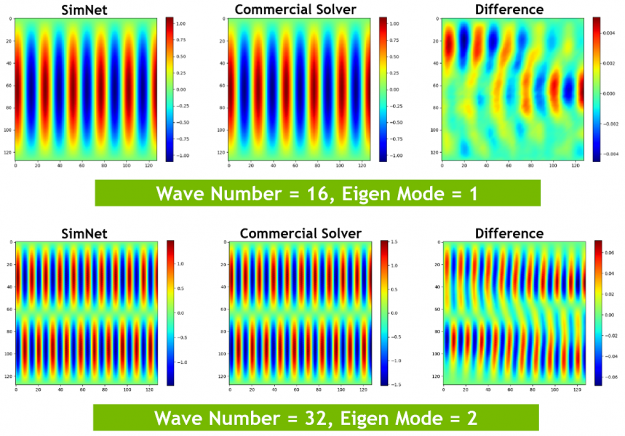
Electromagnetics Frequency domain electromagnetic simulation can be carried out using SimNet v21.06. Solution of real form of frequency domain Maxwell’s equation is available either in scalar form (Helmholtz equation) for 1D, 2D and 3D cases, or in vector form for 3D case. The boundary conditions can be perfect electronic conductor (PEC) for 2D and 3D cases, radiation boundary (absorbing boundary) condition for 3D and waveguide port solver for 2D waveguide source. The implementation can solve for 2D TEz and TMz mode frequency domain electromagnetics and 3D electromagnetics in real form.
Time Stepping Scheme for Temporal Physics Transient simulations are required for many computational problems in such fields as fluid dynamics and electromagnetism. Until recently, neural network solvers have struggled to obtain accurate results. Using several innovations in this field, SimNet is now able solve a variety of transient problems to significantly greater degree of speed and accuracy. Shown below is Taylor-Green vortex decay using transient and turbulent Navier-Stokes simulation.
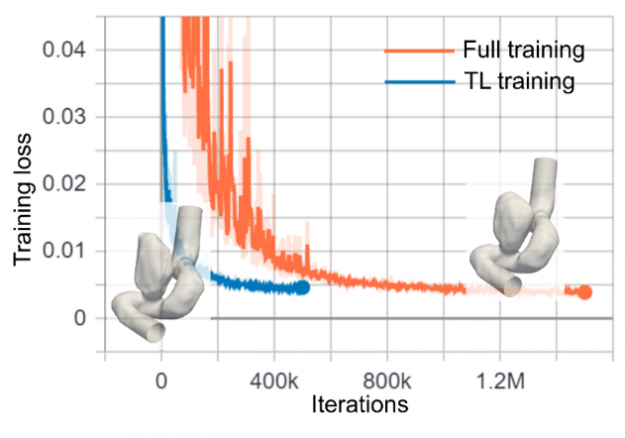
Transfer Learning In repetitive trainings, such as training for surrogate-based design optimization or uncertainty quantification, transfer learning reduces the time to convergence for neural network solvers. Once a model is trained for a single geometry, the trained model parameters are transferred to solve a different geometry, without having to train on the new geometry from scratch.
Transfer learning accelerates patient-specific intracranial aneurysm simulations.
Aneurysms with two different shapes.
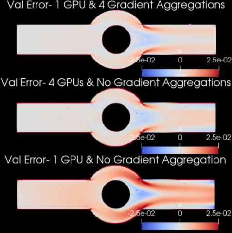
Gradient Aggregation Training of a neural network solver for complex problems requires a large batch size that can be beyond the available GPU memory limits. Increasing the number of GPUs can effectively increase the batch size but in case of limited GPU availability, you can use gradient aggregation. With gradient aggregation, the required gradients are computed in several forward/backward iterations using different mini batches of the point cloud and are then aggregated and applied to update the model parameters. This will, in effect, increase the batch size (although at the cost of increasing the training time).
Increasing the batch size can improve the accuracy of neural network solvers.
4 Gradient Aggregations on 1 GPU = 4 GPUs without Gradient Aggregations. These results are more accurate than the 1 GPU result without any Gradient Aggregation.
Recent SimNet On-Demand Technical Sessions
“Physics-Informed Neural Networks for Mechanics of Heterogenous Media” – IIT-Bombay presented a session on Physics-Informed Neural Networks for Mechanics of Heterogeneous Media. The PINN-based NVIDIA SimNet toolkit is used to develop a framework for the simulation of damage in elastic and elastoplastic materials. For verification, SimNet results are found in good agreement with the analytical solution based on Haghighat et al, 2020.
“Using Physics-Informed Neural Networks and SimNet to Accelerate Product Development” – Kinetic Vision presented a session on using Physics Informed Neural Networks and SimNet to accelerate product development where the Coanda effect, encountered in aerospace and several industrial applications, is simulated using SimNet. Both 2D and 3D geometries are constructed using SimNet’s internal Geometry module and simulated using modified Fourier Network Architecture. The results showed that qualitatively, the velocity flow field predicted by the commercial CFD code, Ansys Fluent and the trained SimNet PINN are very similar. Furthermore, Kinetic Vision did parametric simulations with SimNet and went a step further by taking these results and integrating them into CAD with SolidWorks for automated inference as well as providing a way for users to interact with SimNet from within Solidworks UI.
“Hybrid Physics-Informed Neural Networks for Digital Twin in Prognosis and Health Management” – University of Central Florida presented a session on Hybrid Physics-Informed Neural Networks for Digital Twin in Prognosis and Health Management where a Digital twin model is built to predict damage and fatigue crack growth in aircraft window panels. SimNet models are based in physics and this ensures accuracy needed for prognosis and health management of structural materials. Once SimNet models are trained, they can be used to perform fast and accurate computations as a function of different input conditions. SimNet also achieves good accuracy that the commercial solvers achieve with high degree of mesh refinement. With SimNet, they can scale the predictive model to a fleet of 500 aircraft and get predictions in less than 10 seconds as opposed to taking a few days to weeks if they were to perform the same computations using high-fidelity finite element models.
“Physics-Informed Neural Network for Flow and Transport in Porous Media” – Stanford University presented a session on Physics-Informed Deep Learning for Flow and Transport in Porous Media where a methodology is used to simulate a 2-phase immiscible transport problem (Buckley-Leverett). The model can produce an accurate physical solution both in terms of shock and rarefaction and honors the governing partial differential equation along with initial and boundary conditions. Read more about this on our NVIDIA blog here.
“AI-Accelerated Computational Science and Engineering Using Physics-Based Neural Networks” – NVIDIA presented a session on AI-Accelerated Computational Science and Engineering Using Physics-Based Neural Networks that covers state-of-the-art AI for addressing diverse areas of applications ranging from real-time simulation (e.g., digital twin and autonomous machines) to design space exploration (generative design and product design optimization), inverse problems (e.g., medical imaging, full wave inversion in oil and gas exploration) and improved science (e.g., micromechanics, turbulence) that are difficult to solve because of various gradients and discontinuities, due to physics laws and complex shapes.

 In AI and computer vision, data acquisition is costly and time-consuming and human-based labeling can be error-prone. The accuracy of the models is also affected by insufficient and poorly balanced data and the prolonged time required to improve the deep learning models. It always requires the reacquisition of data in the real world. The collection, …
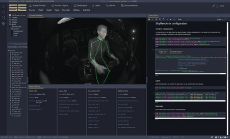

 The long, cumbersome slog of data procurement has been slowing down innovation in AI, especially in computer vision, which relies on labeled images and video for training. But now you can jumpstart your machine learning process by quickly generating synthetic data using AI.Reverie. With the AI.Reverie synthetic data platform, you can create the exact training …
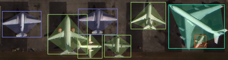
 NVIDIA SimNet is a physics-informed neural network (PINNs) toolkit, which addresses these challenges using AI and physics.