Congratulations. You’ve made it to another awesome GFN Thursday. This year’s Gamescom was full of announcements for GeForce NOW. We’ve got all of the exciting updates for the future of Dying Light 2 Stay Human streaming on GeForce NOW upon release later this year, as well as Marvel’s Guardians of the Galaxy coming with support Read article >
Geometric deep learning is a “program” that aspires to situate deep learning architectures and techniques in a framework of mathematical priors. The priors, such as various types of invariance, first arise in some physical domain. A neural network that well matches the domain will preserve as many invariances as possible. In this post, we present a very conceptual, high-level overview, and highlight a few applications.
Geometric deep learning is a “program” that aspires to situate deep learning architectures and techniques in a framework of mathematical priors. The priors, such as various types of invariance, first arise in some physical domain. A neural network that well matches the domain will preserve as many invariances as possible. In this post, we present a very conceptual, high-level overview, and highlight a few applications.
NVIDIA Triton can manage any number and mix of models (limited by system disk and memory resources). It also supports multiple deep-learning frameworks such as TensorFlow, PyTorch, NVIDIA TensorRT, and so on. This provides flexibility to developers and data scientists, who no longer have to use a specific model framework. NVIDIA Triton is designed to integrate easily with Kubernetes for large-scale deployment in the data center.
NVIDIA Triton Inference Server is an open-source AI model serving software that simplifies the deployment of trained AI models at scale in production. Clients can send inference requests remotely to the provided HTTP or gRPC endpoints for any model managed by the server.
NVIDIA Triton can manage any number and mix of models (limited by system disk and memory resources). It also supports multiple deep-learning frameworks such as TensorFlow, PyTorch, NVIDIA TensorRT, and so on. This provides flexibility to developers and data scientists, who no longer have to use a specific model framework. NVIDIA Triton is designed to integrate easily with Kubernetes for large-scale deployment in the data center.
Multi-Instance GPU (MIG) can maximize the GPU utilization of A100 GPU and the newly announced A30 GPU. It can also enable multiple users to share a single GPU, by running multiple workloads in parallel as if there were multiple, smaller GPUs. MIG capability can divide a single GPU into multiple GPU partitions called GPU instances. Each instance has dedicated memory and compute resources, so the hardware-level isolation ensures simultaneous workload execution with guaranteed quality of service and fault isolation.
In this post, we share the following best practices:
Deploying multiple Triton Inference Servers in parallel using MIG on A100
Autoscaling the number of Triton Inference Servers based on the number of inference requests using Kubernetes and Prometheus monitoring stack.
Using the NGINX Plus load balancer to distribute the inference load evenly among different Triton Inference Servers.
This idea can be applied to multiple A100 or A30 GPUs on a single node or multiple nodes for autoscaling NVIDIA Triton deployment in production. For example, a DGX A100 allows up to 56 Triton Inference Servers (each A100 having up to seven servers using MIG) running on Kubernetes Pods.
Hardware and software prerequisites
To use MIG, you must enable MIG mode and create MIG devices on A100 or A30 GPUs. You can use nvidia-smi to create GPU instances and compute instances manually. Alternately, use the NVIDIA new MIG Parted tool nvidia-mig-parted, which allows administrators to define declaratively a set of possible MIG configurations to be applied to all GPUs on a node.
At runtime, point nvidia-mig-parted at one of these configurations, and nvidia-mig-parted takes care of applying it. In this way, the same configuration file can be spread across all nodes in a cluster, and a runtime flag can be used to decide which of these configurations to be applied to a node. Because the MIG configuration is gone if you reboot the machine, nvidia-mig-parted also makes it easier to create MIG instances after rebooting.
In the Kubernetes environment, you must install the NVIDIA device plug-in and GPU feature discovery plug-in to be able to use MIG. You could install each plug-in separately, or use the cloud-native NVIDIA GPU Operator, which is a single package that includes everything to enable GPU in Kubernetes. You can also use the NVIDIA deployment tool DeepOps, which takes care of installation and plug-ins, and the Prometheus monitoring stack including kube-prometheus, Prometheus, and the Prometheus adapter, that you should use for autoscaling Triton Inference Servers.
You could use either single strategy or mixed strategy for MIG in Kubernetes. In this post, we suggest the mixed strategy, as you have seven MIG devices for one A100 GPU while the other A100 MIG is disabled.
Use the Flower demo, which classifies the images of flowers using ResNet50. The NVIDIA Triton Inference Server container image can be pulled from NGC. Prepare the server’s model files (*.plan, config.pbtxt) and client for the Flower demo. For more information, see Minimizing Deep Learning Inference Latency with NVIDIA Multi-Instance GPU.
Flower demo with Kubernetes
After setting up the flower demo, you want to extend it to a Deployment in a Kubernetes environment. Do this so that the number of Triton Inference Servers can be autoscaled based on the inference requests and the inference load can be distributed among all the servers. Because it allows up to seven MIG devices on an A100, you can have up to seven Kubernetes Pods, each having a Triton Inference Server running on a MIG device. Here are the major steps to deploying Triton Inference Servers with autoscaling and load balancing:
Create a Kubernetes Deployment for Triton Inference Servers.
Create a Kubernetes Service to expose Triton Inference Servers as a network service.
Expose NVIDIA Triton metrics to Prometheus using kube-prometheus and PodMonitor.
Create ConfigMap to define a custom metric.
Deploy Prometheus Adapter and expose the custom metric as a registered Kubernetes APIService.
Create HPA (Horizontal Pod Autoscaler) to use the custom metric.
Use NGINX Plus load balancer to distribute inference requests among all the Triton Inference servers.
The following sections provide the step-by-step guide to achieve these goals.
Create a Kubernetes Deployment for Triton Inference Servers
The first step is to create a Kubernetes Deployment for Triton Inference Servers. A Deployment provides declarative updates for Pods and ReplicaSets. A ReplicaSet in Kubernetes starts multiple instances of the same Pod at the same time.
The following flower-replicas3.yml file creates three replicated Pods, indicated by the .spec.replicas field, which can be any number between one to seven. The .spec.selector field defines how the Deployment finds which Pods to manage. Each Pod runs one container, named flower, which runs the Triton Inference Server image at version 20.12-py3. Same as NVIDIA Triton port numbers, the container ports 8000, 8001, 8002 are reserved for HTTP, gRPC, and NVIDIA Triton metrics, respectively.
The .resources.limits field specifies a MIG device with 5 GB of memory for each Pod using the mixed strategy. The notation nvidia.com/mig-1g.5gb is specific to the mixed strategy and must be adapted accordingly for your Kubernetes cluster. In this example, the model for NVIDIA Triton is stored on a shared file system using NFS protocol. If you do not have a shared file system, you must ensure that the model is loaded to all worker nodes to be accessible by the Pods started by Kubernetes.
Create a Kubernetes Service for Triton Inference Servers
The second step is to create a Kubernetes Service to expose Triton Inference Servers as a network service, so that clients can send inference requests to the servers. When creating a Service, choose the option of automatically creating an external load balancer, as shown in the .type field. This provides an externally accessible IP address that sends traffic to the correct port on the node. The following code example is the flower-service.yml file:
Now the Triton Inference Servers are ready to receive inference requests from the remote clients (Figure 1). If the client sends inference requests, the client can view the classification results of the flower images and also the throughput and end to end latency of each inference request.
Figure 1. (left) Clients sending inference requests to Triton Inference Servers running on MIG devices in Kubernetes. (right) The client getting classification results and performance numbers.
So far, you have multiple Triton Inference Servers running on MIG devices in Kubernetes environments, doing inference on the flower images sent by the client and you can manually change the number of servers. In the next sections, you improve it so that the number of servers can be autoscaled based on the client requests.
Use Prometheus to scrape NVIDIA Triton metrics
To automatically change the number of Triton Inference servers running on Kubernetes Pods, first collect NVIDIA Triton metrics that can be used to define a custom metric. Because there are several sets of NVIDIA Triton metrics from multiple Kubernetes Pods, you should deploy a PodMonitor that tells Prometheus to scrape the metrics from all the Pods.
Prometheus is an open-source, systems monitoring and alerting toolkit that provides time series data identified by metric name and key/value pairs. PromQL, a flexible query language, is used to query metrics from Prometheus.
Create PodMonitor for Prometheus
PodMonitor defines monitoring for a set of Pods, for target discovery by Prometheus. In the flower-pod-monitor.yml file, you define a PodMonitor to monitor the Pods of the servers, as shown in the .spec.selector field. You also need kube-prometheus, which includes the deployment of Prometheus and scrapes the target configuration linking Prometheus to various metrics endpoints, as indicated by the .spec.podMetricsEndpoints field. Prometheus scrapes NVIDIA Triton metrics from these endpoints every 10 seconds, which are defined by the .interval field.
A common problem related to PodMonitor identification by Prometheus is related to incorrect tagging that does not match the Prometheus custom resource definition scope. To match the labels of the NVIDIA Triton Deployment, make sure that the .spec.selector.matchLabels field is app:flower, and the .spec.namespaceSelector.matchNames field is -default. Both should be under the same namespace as the NVIDIA Triton Deployment. This can be confirmed by checking the related labels in the flower-replicas3.yml file. To match the labels of kube-prometheus, also make sure that the .metadata.labels field is release: kube-prometheus-stack. Check the labels using the following commands:
$ kubectl get Prometheus -n monitoring
    NAME                                                 VERSION   REPLICAS   AGE
    kube-prometheus-stack-prometheus   v2.21.0               1          56d
    $ kubectl describe Prometheus kube-prometheus-stack-prometheus -n monitoring
    Name:         kube-prometheus-stack-prometheus
    Namespace:    monitoring
    Labels:       app=kube-prometheus-stack-prometheus
               chart=kube-prometheus-stack-10.0.2
               heritage=Helm
               release=kube-prometheus-stack
    Annotations:
    API Version:  monitoring.coreos.com/v1
    Kind:         Prometheus
    Metadata:
    ……

       Pod Monitor Namespace Selector:
       Pod Monitor Selector:
          Match Labels:
             Release:   kube-prometheus-stack
Deploy the PodMonitor using the command kubectl apply -f flower-pod-monitor.yml and confirm it:
$ kubectl get PodMonitor -n monitoring
     NAME                                                  AGE
     kube-prometheus-stack-tritonmetrics   20s
Query NVIDIA Triton metrics using Prometheus
By default, Prometheus comes with a user interface that can be accessed on port 9090 on the Prometheus server. Open Prometheus in a web browser and choose Status, Targets. You can see that the metrics from three servers are correctly detected by kube-prometheus and added to Prometheus for scrapping.
You can query any NVIDIA Triton metrics such as nv_inference_queue_duration_us or nv_inference_request_success individually or query the following custom metric using PromQL and get the three values calculated by Prometheus (Figure 2). Add avg to get the average value of the three Pods:
When you choose Graph, Prometheus also provides time series data as a graph. We provide more information on this metric in the next section.
Figure 2. Query the custom metric using PromQL in Prometheus graphical user interface
Autoscale Triton Inference Servers
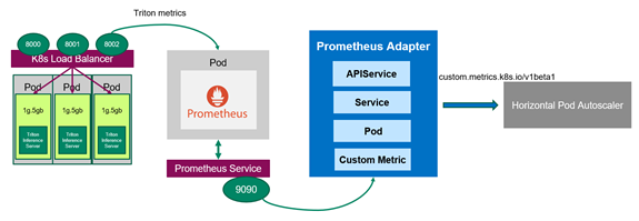
Figure 3. The Prometheus adapter communicates with Kubernetes and Prometheus
Now that you have Prometheus monitoring the servers, you should deploy the Prometheus adapter, which knows how to communicate with both Kubernetes and Prometheus (Figure 3). The adapter helps you use the metrics collected by Prometheus to make scaling decisions. The adapter gathers the names of available metrics from Prometheus at a regular interval and then only exposes metrics that follow specific forms. These metrics are exposed by an API service and can be readily used by HPA.
Optional: Enable permissive binding
In the Kubernetes cluster, role-based access control (RBAC) is a common method to regulate access to different objects. For this example, you must allow the HPA running in a different namespace to access the metrics provided by the metrics API. The configuration for RBAC differs greatly with respect to the configuration of your Kubernetes cluster. For more information about how to use role-based access control, see Using RBAC Authorization.
In the demo, you can create a ClusterRoleBinding object with permissive binding to allow the kubelet user access to all Pods by issuing the following command. This effectively disables any kind of security within your Kubernetes cluster and must not be used for a production environment.
First, tell the Prometheus adapter how to collect a specific metric. You use two NVIDIA Triton metrics to define the custom metric avg_time_queue_us in a ConfigMap for which HPA performs autoscaling. A ConfigMap has a key and the value looks like a fragment of a configuration format. In the ConfigMap file custom-metrics-server-config.yml, the following values are used:
nv_inference_request_success[30] is the number of successful inference requests in the past 30 seconds.
nv_inference_queue_duration_us is the cumulative inference queuing duration in microseconds.
The custom metric means the average queue time per inference request in the past 30 seconds and HPA decides whether to change the replica number based on it.
When configuring the Prometheus adapter, it is important that the metrics have a named endpoint such as a Pod to be addressed to. Unaddressed metrics cannot be queried from the metrics API later. Add the .overrides field to enforce that pod and namespace are exposed in the API later.
apiVersion: v1
 kind: ConfigMap
 metadata:
   name: adapter-config
   namespace: monitoring
 data:
   triton-adapter-config.yml: |
     rules:
     - seriesQuery: 'nv_inference_queue_duration_us{namespace="default",pod!=""}'
       resources:
         overrides:
           namespace:
             resource: "namespace"
           pod:
             resource: "pod"
       name:
         matches: "nv_inference_queue_duration_us"
         as: "avg_time_queue_us"
      metricsQuery: 'avg(delta(nv_inference_queue_duration_us{>}[30s])/
 (1+delta(nv_inference_request_success{>}[30s]))) by (>)'

      Create the ConfigMap and confirm it:
 $ kubectl apply -f custom-metrics-server-config.yml
 configmap/adapter-config created
 $ kubectl get configmap -n monitoring
 NAME                                                      DATA   AGE
 adapter-config                                            1        22s
Create the Prometheus adapter for the Kubernetes metrics API
For the HPA to react to this custom metric, you must create the Kubernetes Deployment, Service, and APIService for the Prometheus adapter. The following code example is the Deployment file, custom-metrics-server-deployment.yml. It uses the ConfigMap from the last step, which tells the adapter to collect the custom metric. It also creates the Deployment that spawns the adapter Pod to pull the custom metric from Prometheus. The .containers.config field must match the .mountPath field and the filename triton-adapter-configl.yml created in the ConfigMap in the previous step.
Create a Kubernetes Service for the Prometheus adapter. In the following file, custom-metrics-server-service.yml, the .spec.selector. field must match the labels app: triton-custom-metris-apiserver in the Deployment, to specify the Pod that provides the Service.
Next, create an APIService so that the Prometheus adapter is accessible by Kubernetes. Then, the custom metric can be fetched by HPA. The following code block is the APIService file custom-metrics-server-apiservice.yml. The .spec.service field must match the .metadata field of the Service file. To allow the autoscaler to access the custom metric, you should register the metric with the API aggregator. The required API to use here is custom.metrics.k8s.io/v1beta1.
Before you deploy the Prometheus adapter, you can see that no metrics are available at the API point:
 $ kubectl get --raw "/apis/custom.metrics.k8s.io/v1beta1" | jq
 Error from server (NotFound): the server could not find the requested resource
Use the command kubectl apply to apply the configuration in the three .yml files previously mentioned. After you create the APIService for the Prometheus adapter, you can see that the custom metric is available:
You can also check the current value of this custom metric, which is 0 as there is currently no inference request from the client. Here, you are selecting all Pods from the default namespace, in which the flower-demo is deployed:
The HPA autoscales the number of Pods in a replication controller, Deployment, ReplicaSet, or stateful set based on observed metrics. Now you can create an HPA that uses the custom metric. The HPA controls the number of replicas deployed in Kubernetes according to the following equation. It operates on the ratio between desired metric value and current metric value and returns the number of desired replicas:
In this formula, the following are used:
is the number of replicas that Kubernetes has.
is the current number of replicas.
is the current metric: the average of the custom metric values from all servers in this case.
is the desired metric value.
When is different from CR, HPA increases or decreases the number of replicas by acting on the Kubernetes Deployment (Pods). Basically, whenever the ratio between the current metric value and the desired metric value is larger than 1, then new replicas can be deployed.
Figure 4. HPA scales NVIDIA Triton Deployment
The following HPA file flower-hpa.yml autoscales the Deployment of Triton Inference Servers. It uses a Pods metric indicated by the .sepc.metrics field, which takes the average of the given metric across all the Pods controlled by the autoscaling target. The .spec.metrics.targetAverageValue field is specified by considering the value ranges of the custom metric from all the Pods. The field triggers HPA to adjust the number of replicas periodically to match the observed custom metric with the target value.
Create the HPA using the command kubectl apply -f flower-hpa.yml and confirm it:
 $ kubectl get hpa
 NAME         REFERENCE      TARGETS   MINPODS   MAXPODS   REPLICAS   AGE
 flower-hpa   Deployment/flower   0/50              1                 7                    1              22s
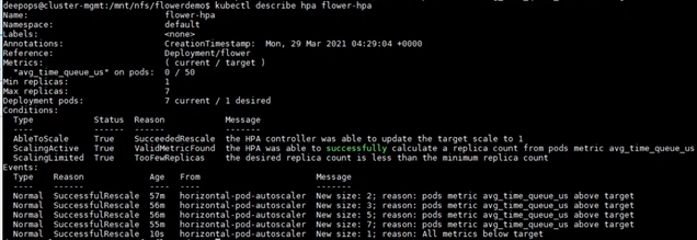
If clients start sending inference requests to the servers, the new HPA can pick up the custom metric for the Deployment and establish the needed number of Pods. For example, when there are increasing inference requests, HPA increases the number of Pods from 1 to 2, and gradually to 7, which is the maximum number of Pods on an A100 GPU. Finally, when the clients stop sending inference requests, HPA decreases the Replica number to only 1 (Figure 5).
Figure 5. Using the command kubectl describe hpa flower-hpa to check how HPA increase or decrease the number of Pods.
Load balance with NGINX Plus
Load balancing is for distributing the load from clients optimally across available servers. Earlier, you chose the Kubernetes built-in load balancer, a Layer 4 (transport layer) load balancer, which is easy to deploy but with the limitation using gRPC.
In this demo, using Prometheus, you find that the Pods newly added by the autoscaler cannot get the workload using Kubernetes built-in load balancer. To improve this, use NGINX Plus, which is a Layer 7 (application layer) load balancer. The workload is evenly distributed among all the Pods, including the newly scaled-up Pods.
First, you should create an NGINX Plus image because a commercial offering of NGINX Plus is not available from Docker Hub. Create an NGINX instance in a Docker container using the NGINX open source image from Docker Hub. Then, push the local image to a private Docker registry.
Next, to deploy NGINX Plus, label the node on which to deploy NGINX Plus with role=nginxplususing the following command:
$ kubectl label node role=nginxplus
Modify the Service to set clusterIP to none, so that all the replicas endpoints are exposed and identified by NGINX Plus. To avoid confusion, create a new Service file, flower-service-nginx.yml, and apply it:
Next, create a configuration file for NGINX. The following code example assumes that you are using the location /path/to/nginx/config/nginx.conf.
 resolver  valid=5s;
 upstream backend {
    zone upstream-backend 64k;
    server  resolve;
 }

 upstream backendgrpc {
    zone upstream-backend 64k;
    server  resolve;
 }

 server {
    listen 80;
    status_zone backend-servers;

    location / {
      proxy_pass http://backend;
      health_check uri=/v2/health/ready;
    }
 }

 server {
         listen 89 http2;

         location / {
             grpc_pass grpc://backendgrpc;
         }
 }

 server {
     listen 8080;
     root /usr/share/nginx/html;
     location = /dashboard.html { }
     location = / {
        return 302 /dashboard.html;
     }
     location /api {
       api write=on;
     }
 }
Lastly, you should create a ReplicationController for NGINX Plus in the following nginxplus-rc.yml file. To pull the image from the private registry, Kubernetes needs credentials. The imagePullSecrets field in the configuration file specifies that Kubernetes should get the credentials from a Secret named regcred. In this configuration file, you must also mount the NGINX config file created in the last step to the location /etc/nginx/conf.d.
Create the ReplicationController using the following command:
kubectl create -f nginxplus-rc.yml
Verify the Deployment. You should find that NGINX Plus is running:
 $kubectl get pods
 NAME                      READY   STATUS    RESTARTS   AGE
 flower-5cf8b78894-jng2g   1/1     Running   0          8h
 nginxplus-rc-nvj7b        1/1     Running   0          10s
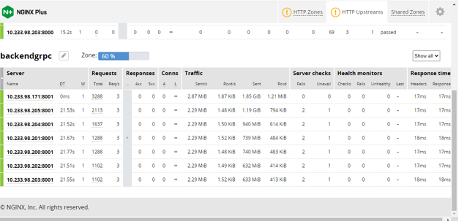
Now when clients send inference requests to the servers, you can see the NGINX Plus Dashboard (Figure 6):
The autoscaler increases the number of Pods gradually from one to seven.
The workload is evenly distributed among all the Pods, as shown in Traffic.
You can also confirm that the newly added Pods are busy working by checking the values of the metrics or custom metric from all the Pods in Prometheus.
Figure 6. NGINX Plus dashboard showing the number of NVIDIA Triton servers scaled by HPA and each server’s information.
Conclusion
This post showed the step-by-step instructions and code to deploy Triton Inference Servers at a large scale with MIG in a Kubernetes environment. We also showed you how to autoscale the number of servers and balance the workload using two different types of load balancers. We recorded all the steps and results and you can also watch the Triton Deployment at Scale with Multi-Instance-GPU (MIG) and Kubernetes GTC’21 session.
NVIDIA DRIVE OS 5.2.6 Linux SDK is now available on the NVIDIA DRIVE Developer site, providing developers with the latest operating system and development environment purpose-built for autonomous vehicles. As the foundation of the NVIDIA DRIVE SDK, NVIDIA DRIVE OS is designed specifically for accelerated computing and artificial intelligence. It includes NVIDIA CUDA for efficient … Continued
NVIDIA DRIVE OS 5.2.6 Linux SDK is now available on the NVIDIA DRIVE Developer site, providing developers with the latest operating system and development environment purpose-built for autonomous vehicles.
As the foundation of the NVIDIA DRIVE SDK, NVIDIA DRIVE OS is designed specifically for accelerated computing and artificial intelligence. It includes NVIDIA CUDA for efficient parallel computing, NVIDIA TensorRT for real-time AI inference, NvMedia for sensor input processing, and specialized developer tools and modules that allow developers to optimize performance for DRIVE AGX hardware accelerated engines.
And with this latest release, NVIDIA DRIVE Platform Docker containers are now available to members of the NVIDIA DRIVE Developer Program on NVIDIA GPU Cloud (NGC) for beta testing. Docker for DRIVE Development enables host independence, isolation, multiple SDK versions, as well as a consistent environment.
Developers can install the latest version of NVIDIA DRIVE OS 5.2.6 Linux by following the Install DRIVE OS with SDK Manager instructions in the DRIVE OS 5.2.6 Installation Guide.
NVIDIA DRIVE OS 5.2.6 Linux features include:
NVIDIA DRIVE Platform Docker Containers (Beta)
DRIVE OS Linux designated for use in production environment
Efficient image processing through NvSIPL framework
SSH enabled by default on the target
Persistent storage of user login on the target (i.e., username/password, SSH keys)
Please register for an NVIDIA Developer account and apply for membership in the Developer Program before proceeding. See the DRIVE OS 5.2.6 Installation Guide for registration and installation information and please submit questions or feedback on the Docker containers to the DRIVE AGX General Forum. We want your feedback!
And be sure to check out the new DRIVE Download page, where developers can easily find relevant solutions for robust autonomous driving development.
Learn about the latest additions and software updates to the NVIDIA NGC catalog, a hub of GPU-optimized software that simplifies and accelerates workflows.
The NVIDIA NGC catalog is a hub for GPU-optimized deep learning, machine learning, and HPC applications. With highly performant software containers, pretrained models, industry-specific SDKs, and Helm Charts the content available on the catalog helps simplify and accelerate end-to-end workflows.
A few additions and software updates to the NGC catalog include:
NVIDIA NeMo
NVIDIA NeMo (Neural Modules) is an open source toolkit for conversational AI. It is designed for data scientists and researchers to build new state-of-the-art speech and NLP networks easily through API compatible building blocks that can be connected.
The latest version of NeMo adds support for Conformer ONNX conversion and streaming inference of long AU files, and improves performance of speaker clustering, verification, and diarization. Furthermore, it adds multiple datasets, right to left models, noisy channel reranking, ensembling for NMT. It also improves NMT training efficiency and adds tutorial notebooks for NMT data cleaning and preprocessing.
NVIDIA HPC SDK
The NVIDIA HPC SDK is a comprehensive suite of compilers, libraries, and tools essential to maximizing developer productivity, performance, and portability of HPC applications.
The latest version includes full support for the NVIDIA Arm HPC Developer Kit and CUDA 11.4. It also offers HPC compilers with Arm-specific performance enhancements, including improved vectorization and optimized math functions.
NVIDIA Data Center Infrastructure-on-a-Chip Architecture (NVIDIA DOCA)
The NVIDIA DOCA SDK enables developers to rapidly create applications and services on top of BlueField data processing units (DPUs).
The NVIDIA DOCA container and resource helps deploy NVIDIA DOCA applications and development setups on the BlueField DPU. The deployment is based on Kubernetes and this resource bundles ready-to-use .yaml configuration files required for the different DOCA containers.
NVIDIA System Management (NVSM)
NVSM is a software framework for monitoring DGX nodes in a data center and provides active health monitoring, system alerts, and log generation. NVSM provides DGX Stations the health of the system and diagnostic information.
Deep Learning Software
Our most popular deep learning frameworks for training and inference are updated monthly. Pull the latest version (v21.07) of:
PyTorch Lightning is a lightweight framework for training models at scale, on multi-GPU, multi-node configurations. It does so without changing your code, and turns on advanced training optimizations with a switch of a flag.
The v1.4.0 adds support for Fully Sharded Parallelism, and fits much larger models onto multiple GPUs into memory, reaching over 40 billion parameters on an A100.
Additionally, it supports the new DeepSpeed Infinity plug-in and new cluster environments including KubeflowEnvironment and LSFEnvironment.
At GE Renewable Energy, CTO Danielle Merfeld and technical leader Arvind Rangarajan are making wind, er, mind-blowing advances throughout renewable energy. Merfeld and Rangarajan spoke with NVIDIA AI Podcast host Noah Kravitz about how the company uses AI and a human-in-the-loop process to make renewable energy more widespread. The AI Podcast · GE’s Danielle Merfeld Read article >
Largest GPU-Powered Supercomputer for U.S. Department of Energy’s Argonne Lab Will Enable Scientific Breakthroughs in Era of Exascale AISANTA CLARA, Calif., Aug. 25, 2021 (GLOBE NEWSWIRE) — …
SE(3)-Transformers are versatile graph neural networks unveiled at NeurIPS 2020. NVIDIA just released an open-source optimized implementation that uses 9x less memory and is up to 21x faster than the baseline official implementation. SE(3)-Transformers are useful in dealing with problems with geometric symmetries, like small molecules processing, protein refinement, or point cloud applications. They can … Continued
SE(3)-Transformers are useful in dealing with problems with geometric symmetries, like small molecules processing, protein refinement, or point cloud applications. They can be part of larger drug discovery models, like RoseTTAFold and this replication of AlphaFold2. They can also be used as standalone networks for point cloud classification and molecular property prediction (Figure 1).
Figure 1. Architecture of a typical SE(3)-Transformer used for molecular property prediction.
In the /PyTorch/DrugDiscovery/SE3Transformer repository, NVIDIA provides a recipe to train the optimized model for molecular property prediction tasks on the QM9 dataset. The QM9 dataset contains more than 100k small organic molecules and associated quantum chemical properties.
A 21x higher training throughput
The NVIDIA implementation provides much faster training and inference overall compared with the baseline implementation. This implementation introduces optimizations to the core component of SE(3)-Transformers, namely tensor field networks (TFN), as well as to the self-attention mechanism in graphs.
These optimizations mostly take a form of fusion of operations, given that some conditions on the hyperparameters of attention layers are met.
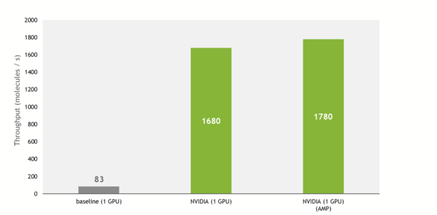
Thanks to these, the training throughput is increased by up to 21x compared to the baseline implementation, taking advantage of Tensor Cores on recent NVIDIA GPUs.
Figure 2. Training throughput on an A100 GPU. QM9 dataset with a batch size of 100.
In addition, the NVIDIA implementation allows the use of multiple GPUs to train the model in a data-parallel way, fully using the compute power of a DGX A100 (8x A100 80GB).
Putting everything together, on an NVIDIA DGX A100, SE(3)-Transformers can now be trained in 27 minutes on the QM9 dataset. As a comparison, the authors of the original paper state that the training took 2.5 days on their hardware (NVIDIA GeForce GTX 1080 Ti).
Faster training enables you to iterate quickly during the search for the optimal architecture. Together with the lower memory usage, you can now train bigger models with more attention layers or hidden channels, and feed larger inputs to the model.
A 9x lower memory footprint
SE(3)-Transformers were known to be memory-heavy models, meaning that feeding large inputs like large proteins or many batched small molecules was challenging. This was a bottleneck for users with limited GPU memory.
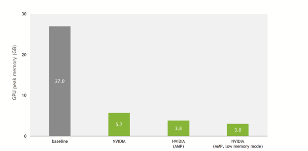
This has now changed with the NVIDIA implementation, open-sourced on DeepLearningExamples. Figure 3 shows that, thanks to NVIDIA optimizations and support for mixed precision, the training memory usage is reduced by up to 9x compared to the baseline implementation.
Figure 3. Comparison of training peak memory consumption between the baseline implementation and NVIDIA implementation of SE(3)-Transformers. Using 100 molecules per batch on the QM9 dataset. V100 32-GB GPU.
In addition to the improvements done for single and mixed precision, a low-memory mode is provided. When this flag is enabled, and the model runs either on TF32 (NVIDIA Ampere Architecture) or FP16 (NVIDIA Ampere Architecture, NVIDIA Turing Architecture, and NVIDIA Volta Architecture) precisions, the model switches to a mode that trades throughput for extra memory savings.
In practice, on the QM9 dataset with a V100 32-GB GPU, the baseline implementation can scale up to a batch size of 100 before running out of memory. The NVIDIA implementation can fit up to 1000 molecules per batch (mixed precision, low-memory mode).
For researchers handling proteins with amino acid residue as nodes, this means that you can feed longer sequences and increase the receptive field of each residue.
SE(3)-Transformer optimizations
Here are some of the optimizations that the NVIDIA implementation provides compared to the baseline. For more information, see the source code and documentation on the DeepLearningExamples/PyTorch/DrugDiscovery/SE3Transformer repository.
Fused keys and values computation
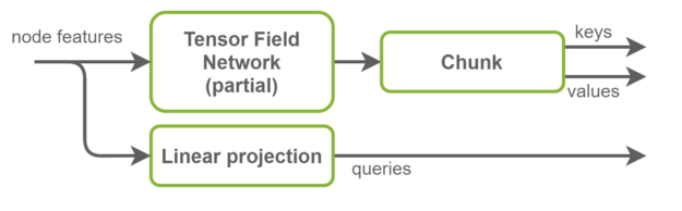
Inside the self-attention layers, keys, queries, and values tensors are computed. Queries are graph node features and are a linear projection of the input features. Keys and values, on the other hand, are graph edge features. They are computed using TFN layers. This is where most computation happens in SE(3)-Transformers and where most of the parameters live.
The baseline implementation uses two separate TFN layers to compute keys and values. In the NVIDIA implementation, those are fused together in one TFN with the number of channels doubled. This reduces by half the number of small CUDA kernels launched, and better exploits GPU parallelism. Radial profiles, which are fully connected networks inside TFNs, are also fused with this optimization. An overview is shown in Figure 4.
Figure 4. Keys, queries, and values computation inside the NVIDIA implementation. Keys and values are computed together and then chunked along the channel dimension.
Fused TFNs
Features inside SE(3)-Transformers have, in addition to their number of channels, a degree, which is a positive integer. A feature of degree has a dimensionality of . A TFN takes in features of different degrees, combines them using tensor products, and outputs features of different degrees.
For a layer with 4 degrees as input and 4 degrees as output, all combinations of degrees are considered: there are in theory 4×4=16 sublayers that must be computed.
These sublayers are called pairwise TFN convolutions. Figure 5 shows an overview of the sublayers involved, along with the input and output dimensionality for each. Contributions to a given output degree (columns) are summed together to obtain the final features.
Figure 5. Pairwise convolutions involved in a TFN layer with 4 degrees as input and 4 degrees as output.
NVIDIA provides multiple levels of fusion to accelerate these convolutions when some conditions on the TFN layers are met. Fused layers enable Tensor Cores to be used more effectively by creating shapes with dimensions being multiples of 16. Here are three cases where fused convolutions are applied:
Output features have the same number of channels
Input features have the same number of channels
Both conditions are true
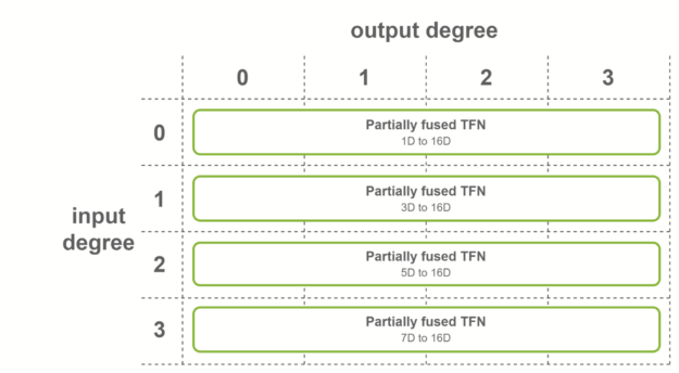
The first case is when all the output features have the same number of channels, and output degrees span the range from 0 to the maximum degree. In this case, fused convolutions that output fused features are used. This fusion level is used for the first TFN layer of SE(3)-Transformers.
Figure 6. Partially fused TFN per output degree.
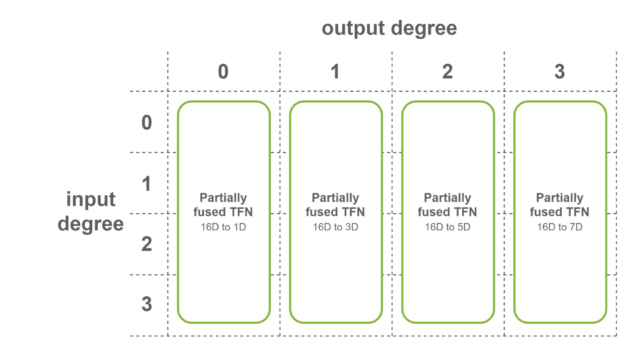
The second case is when all the input features have the same number of channels, and input degrees span the range from 0 to the maximum degree. In this case, fused convolutions that operate on fused input features are used. This fusion level is used for the last TFN layer of SE(3)-Transformers.
Figure 7. Partially fused TFN per input degree.
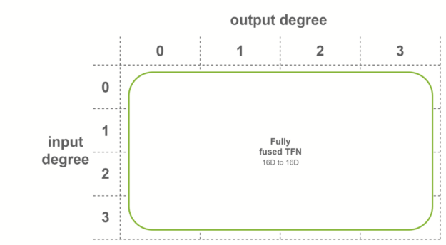
In the last case, fully fused convolutions are used when both conditions are met. These convolutions take as input fused features, and output fused features. This means that only one sublayer is necessary per TFN layer. Internal TFN layers use this fusion level.
Figure 8. Fully fused TFN
Base precomputation
In addition to input node features, TFNs need basis matrices as input. There exists a set of matrices for each graph edge, and these matrices depend on the relative positions between the destination and source nodes.
In the baseline implementation, these matrices are computed in the beginning of the forward pass and shared across all TFN layers. They depend on spherical harmonics, which can be expensive to compute. Because the input graphs do not change (no data augmentation, no iterative position refinement) with the QM9 dataset, this introduces redundant computation across epochs.
The NVIDIA implementation provides the option to precompute those bases at the beginning of the training. The full dataset is iterated one time and the bases are cached in RAM. The process of computing bases at the beginning of forward passes is replaced by a faster CPU to GPU memory copy.
Conclusion
I encourage you to check the implementation of the SE(3)-Transformer model in the NVIDIA /PyTorch/DrugDiscovery/SE3Transformer GitHub repository. In the comments, share how you plan to adopt and extend this project.
The release of NVIDIA Clara Parabricks v3.6 brings new applications for variant calling, annotation, filtering, and quality control to its suite of powerful genomic analysis tools. Now featuring over 33 accelerated tools for every stage of genomic analysis, NVIDIA Clara Parabricks provides GPU-accelerated bioinformatic pipelines that can scale for any workload. As genomes and exomes … Continued
The release of NVIDIA Clara Parabricks v3.6 brings new applications for variant calling, annotation, filtering, and quality control to its suite of powerful genomic analysis tools. Now featuring over 33 accelerated tools for every stage of genomic analysis, NVIDIA Clara Parabricks provides GPU-accelerated bioinformatic pipelines that can scale for any workload.
As genomes and exomes are sequenced at faster speeds than ever before, increasing loads of raw instrument data must be mapped, aligned, and interpreted to decipher variants and their significance to disease. Bioinformatic pipelines need to keep up with genomic analysis tools. CPU-based analysis pipelines often take weeks or months to glean results, while GPU-based pipelines can analyze 30X whole human genomes in 22 minutes and whole human exomes in 4 minutes.
These fast turnaround times are necessary to keep pace with next generation sequencing (NGS) genomic instrument outputs. This is imperative for large-scale population, cancer center, pharmaceutical drug development, and genomic research projects that require quick results for publications.
NVIDIA Clara Parabricks v3.6 Incorporates:
New GPU-accelerated variant callers
An easy-to-use vote-based VCF merging tool (VBVM)
A database annotation tool (VCFANNO)
A new tool for quickly filtering a VCF by allele frequency (FrequencyFiltration)
Tools for VCF quality control (VCFQC and VCFQCbyBAM) for both somatic and germline pipelines.
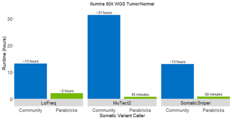
Figure 1: Analysis runtimes for open-source CPU-based somatic variant calling tools compared to GPU-accelerated NVIDIA Clara Parabricks. Relative to the community versions, NVIDIA Clara Parabricks accelerates LoFreq by 6x, SomaticSniper by 16x, and Mutect2 by 42x. These benchmarks were run on 50X WGS matched tumor-normal data from the SEQC-II benchmark set on 4x V100s.
Accelerating LoFreq and Other Somatic Callers
With the addition of LoFreq alongside Strelka2, Mutect2, and SomaticSniper, Clara Parabricks now includes 4 somatic callers for cancer workflows. LoFreq is a fast and sensitive variant caller for inferring SNVs and indels from NGS data. LoFreq runs on a variety of aligned sequencing data such as Illumina, IonTorrent, and Pacbio. It can automatically adapt to changes in coverage and sequencing quality, and can be applied to somatic, viral/quasispecies, metagenomic, and bacterial datasets.
The Lofreq somatic caller in Clara Parabricks is 10X faster compared to its native instance and is ideal for calling low frequency mutations.Using base-call qualities and other sources of errors inherent in NGS data, LoFreq improves the accuracy for calling somatic mutations below the 10% allele frequency threshold.
The accelerated LoFreq supports only SNV calling in v3.6, with Indel calling coming in a subsequent release. Read more >>
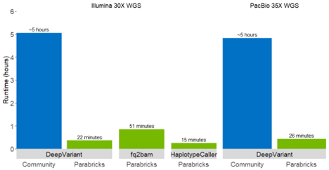
Figure 2: Runtimes for open-source DeepVariant (blue) and GPU-accelerated NVIDIA Clara Parabricks (green). Runtimes for 30X Illumina short read data are on the left; runtimes for PacBio 35X long read data are on the right. NVIDIA Clara Parabricks’ DeepVariant is 10-15x faster than the open-source version (blue “DeepVariant” bars compared to green “DeepVariant” bars).
From Months to Hours with New Accelerated Tools
NVIDIA Clara Parabricks v3.6 also includes a bam2fastq tool, the addition of smoove variant callers, support for de novo mutations, and new tools for VCF processing (for example annotation, filtering, and merging). A standard WGS analysis for a 30x human genome finishes in 22 minutes on a DGX A100, which is over 80 times faster than CPU-based workflows on the same server. With this acceleration, projects taking months can now be done in hours.
Bam2Fastq is an accelerated version of GATK Sam2fastq. It converts a BAM or CRAM file to FASTQ. This is useful for scenarios where samples need to be realigned to a new reference, but the original FASTQs were deleted to save on storage space. Now they can be regenerated from the BAMs and aligned to a new reference more quickly than ever before
Detection of de novo variants (DNVs) that occur in the germline genome when comparing sequence data for an offspring to its parents (aka trio analysis) is critical for studies of disease-related variation, along with creating a baseline for generational mutation rates.
A GPU-based workflow to call DNVs is now included in NVIDIA Clara Parabricks v3.6 and utilizes Google’s DeepVariant, which has been tested on trio analyses and other pedigree sequencing projects. Learn more >>
For structural variant calling, NVIDIA Clara Parabricks already includes Manta, and now smoove has been added. Smoove simplifies and speeds calling and genotyping structural variants for short reads. It also improves specificity by removing alignment signals indicative of low-level noise and often contribute to spurious calls. Learn more >>
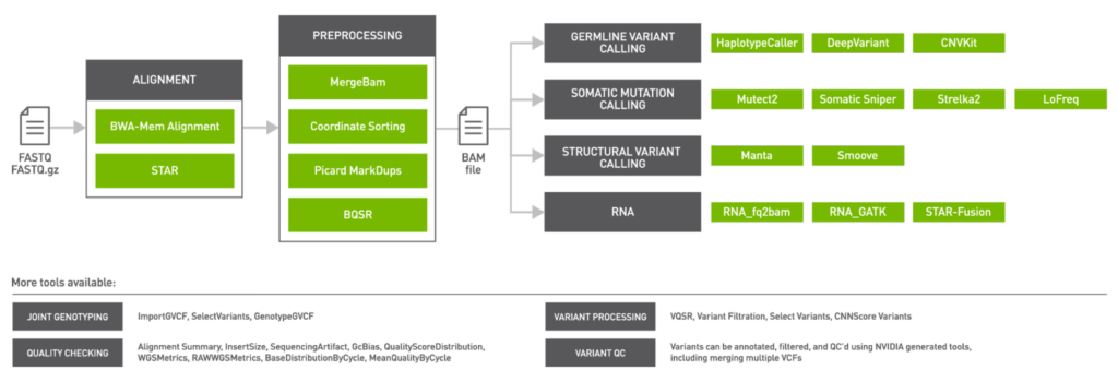
Figure 3: GPU-accelerated genomics analysis tools in NVIDIA Clara Parabricks v3.6.
NVIDIA Clara Parabricks v3.6 also focuses on steps of the genomic pipeline after variant calling. BamBasedVCFQC is an NVIDIA-generated tool to help QC VCF outputs by using SamTools mPileUp results, using the original BAM. Vcfanno allows users to annotate VCF outputs using third-party data sources like dbSNP, adding allele frequencies to the VCF.
FrequencyFiltration allows variants within a VCF to be filtered based upon numeric fields containing allele frequency and read count information. Finally, vote-based somatic caller merger (vbvm) is for merging two or more VCF files and then filtering variants based upon a simple voting-based mechanism where variants can be filtered based upon the number of somatic callers that have identified a specific variant.
Try out the NVIDIA Clara Parabricks GPU-accelerated genomic analysis tools for your germline, cancer, and RNA-Seq analysis workflows for free with a 90-day trial license >>>
Access NVIDIA Clara Parabricks on premise or in the cloud through the AWS Marketplace >>>


 NVIDIA Triton can manage any number and mix of models (limited by system disk and memory resources). It also supports multiple deep-learning frameworks such as TensorFlow, PyTorch, NVIDIA TensorRT, and so on. This provides flexibility to developers and data scientists, who no longer have to use a specific model framework. NVIDIA Triton is designed to integrate easily with Kubernetes for large-scale deployment in the data center.
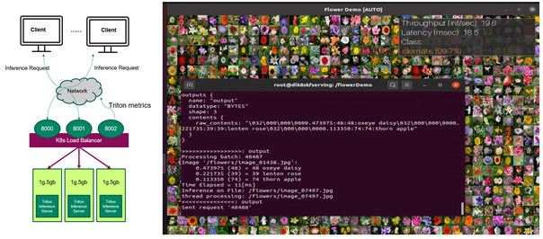
![Prometheus can calculate the three values of the customer metric from three Pods.]](https://developer-blogs.nvidia.com/wp-content/uploads/2021/06/promql-query.png)

 is the number of replicas that Kubernetes has.
 is the current number of replicas.
 is the current metric: the average of the custom metric values from all servers in this case.
 is the desired metric value.
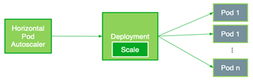
 NVIDIA DRIVE OS 5.2.6 Linux SDK is now available on the NVIDIA DRIVE Developer site, providing developers with the latest operating system and development environment purpose-built for autonomous vehicles. As the foundation of the NVIDIA DRIVE SDK, NVIDIA DRIVE OS is designed specifically for accelerated computing and artificial intelligence. It includes NVIDIA CUDA for efficient …
  Learn about the latest additions and software updates to the NVIDIA NGC catalog, a hub of GPU-optimized software that simplifies and accelerates workflows.
  SE(3)-Transformers are versatile graph neural networks unveiled at NeurIPS 2020. NVIDIA just released an open-source optimized implementation that uses 9x less memory and is up to 21x faster than the baseline official implementation. SE(3)-Transformers are useful in dealing with problems with geometric symmetries, like small molecules processing, protein refinement, or point cloud applications. They can …
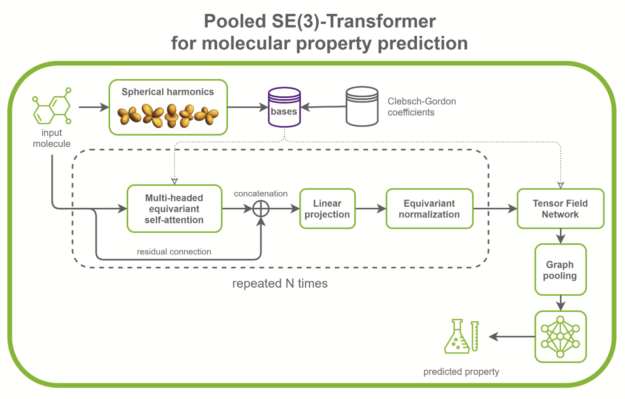
 , which is a positive integer. A feature of degree has a dimensionality
  of . A TFN takes in features of different degrees, combines them using
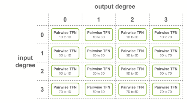
 The release of NVIDIA Clara Parabricks v3.6 brings new applications for variant calling, annotation, filtering, and quality control to its suite of powerful genomic analysis tools. Now featuring over 33 accelerated tools for every stage of genomic analysis, NVIDIA Clara Parabricks provides GPU-accelerated bioinformatic pipelines that can scale for any workload. As genomes and exomes …