Rendering in Real Time with Spatiotemporal Blue Noise Textures, Part 1

Blue noise textures are used in a variety of real time–rendering techniques to hide noise in a perceptually pleasing way

Blue noise textures are useful for providing per-pixel random values to make noise patterns in renderings. Blue noise textures are harder to see and easier to remove than noise made by either random number generators or hashes, both being white noise. To use a blue noise texture, you tile it across the screen, read the texture with nearest neighbor point sampling, and use that as your random value.

In this post, we add the time axis to blue-noise textures, giving each frame high-quality spatial blue noise and making each pixel be blue over time. This provides better convergence and temporal stability over other blue-noise animation methods. We also show you how to make non-uniform blue noise textures to allow for importance sampling. We go on a deeper technical dive in the follow up post, Rendering in Real Time with Spatiotemporal Blue Noise Textures, Part 2.

While other methods combine blue noise and better convergence, they focus on convergence first and blue noise second. Our work focuses on blue noise first and convergence second, which makes for better renders at the lowest of sample counts, where blue noise has the most benefit.

A notable limitation to blue noise textures is that they work best in low-sample-count, low-dimension algorithms. For high sample counts, or high dimensions found in algorithms like path tracing, you would likely want to switch to low-discrepancy sequences to remove the error, instead of trying to hide it with blue noise.

Also worth mentioning is that that pixels under motion under TAA lose temporal benefits and our noise then functions as purely spatial blue noise. Pixels that are still even for a moment gain temporal stability and lower error, however, which is then carried around by TAA when they are in motion again. In these situations, our noise does no worse than spatial blue noise, so it should always be used instead, to gain benefits where available and do no worse otherwise.

For more information, download spatiotemporal blue noise textures and generation code at NVIDIAGameWorks/SpatiotemporalBlueNoiseSDK on GitHub.

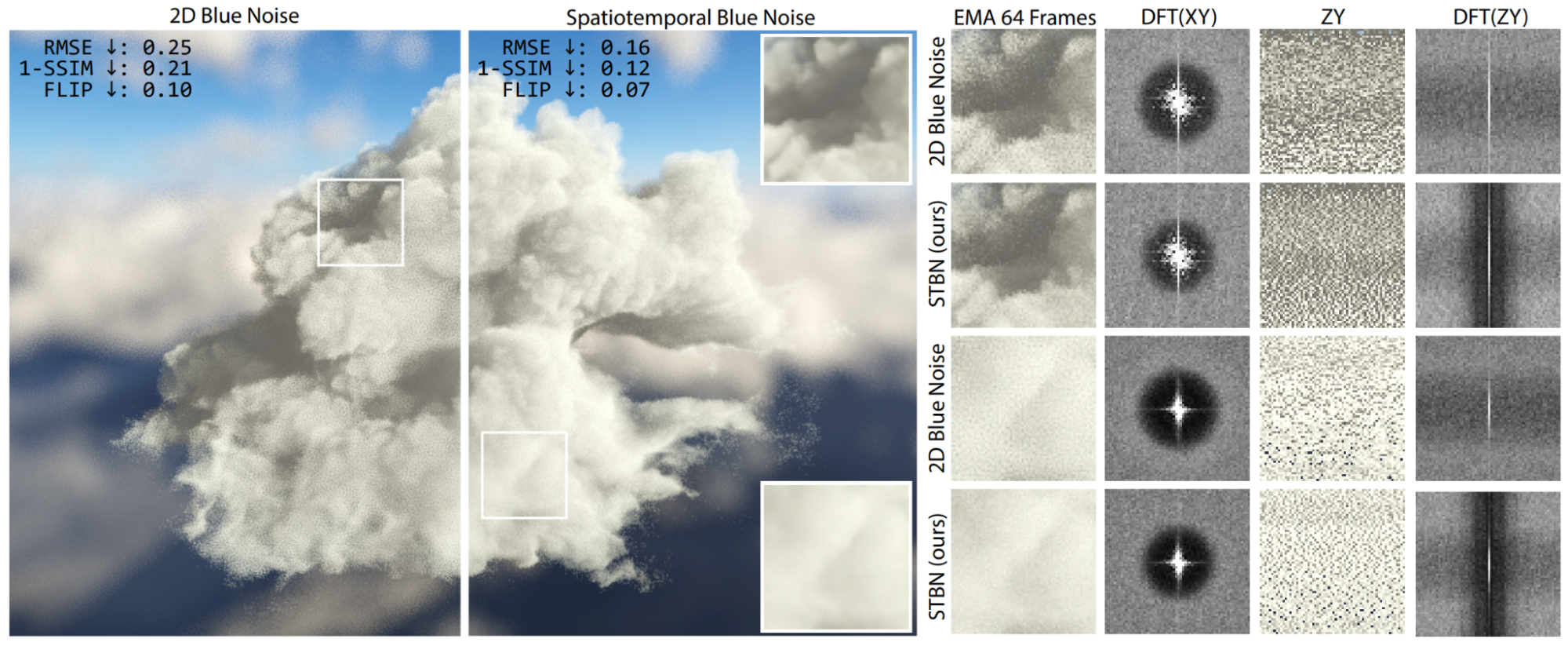
Figure 1 shows an example of using blue noise compared to spatiotemporal blue noise.

Figure 1 uses stochastic single scattering, where free-flight distances are sampled using a series of blue noise masks over time. Traditional 2D blue noise masks (far left) are easy to filter spatially, but exhibit a white noise signal over time, making the underlying signal difficult to filter temporally.

Our spatiotemporal blue noise (STBN) masks (right of large image) additionally exhibit blue noise in the temporal dimension, resulting in a signal that is easier to filter over time. On the far right, we show two crops of the main image, as well as their corresponding discrete Fourier transforms over both space (DFT(XY)) and time (DFT(ZY)). The Z axis is time. The ground truth is shown in the insets in the large image (upper and lower right corners).

Scalars

Scalar spatiotemporal blue noise textures store a scalar value per pixel and are useful for rendering algorithms that want a random scalar value per pixel, such as stochastic transparency. You generate these textures by running the void and cluster algorithm in 3D but modify the energy function.

When calculating the energy between two pixels, you only return the energy value if the two pixels are from the same texture slice (have the same z value) or if they are the same pixel at different points in time (have the same xy value); otherwise, it returns zero. The result is N textures, which are perfectly blue over space, but each pixel individually is also blue over the z axis (time). In these textures, the (x,y) planes are spatial dimensions that correspond to screen pixels, and the z axis is the dimension of time. You advance one step down the z dimension each frame.

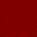
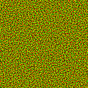
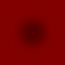
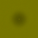
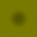
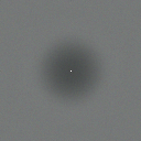
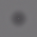
Figure 2 shows example textures and the XY and XZ DFTs for the spatiotemporal blue noise, an array of independent 2D blue noise textures, and 3D blue noise. Only our noise is blue over space (XY) and blue over time (Z), as you can see by the darkening of the center, where the low frequencies are attenuated.

In Figure 2, individual slices of 3D blue noise are not good over space, nor over time. Only our spatiotemporal blue noise is blue over both space and time. For more information about why 3D blue noise is not useful for animating blue noise, see Christoph Peters’ nice explanation in The problem with 3D blue noise.

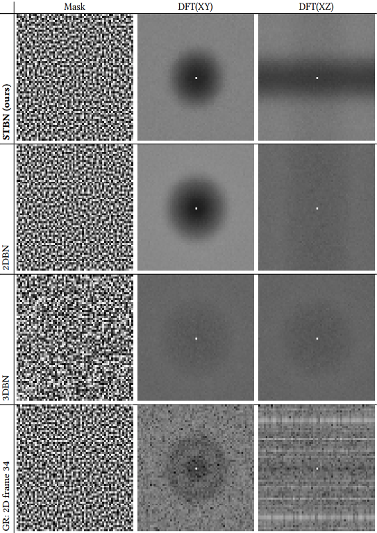
Figure 3 shows a texture that is 50% transparent over a black background, using noise to do a binary alpha test (stochastic transparency) and filtered with temporal anti-aliasing (TAA).

Independent blue noise textures are a significant improvement over white noise by having an evenly spaced set of surviving pixels each frame. This is better for neighborhood sampling rejection, compared to white noise, which has clumps and voids of surviving pixels. Spatiotemporal blue noise does even better by making each pixel survive on frames that are evenly spaced temporally as well, making for a more converged, and more temporally stable result.

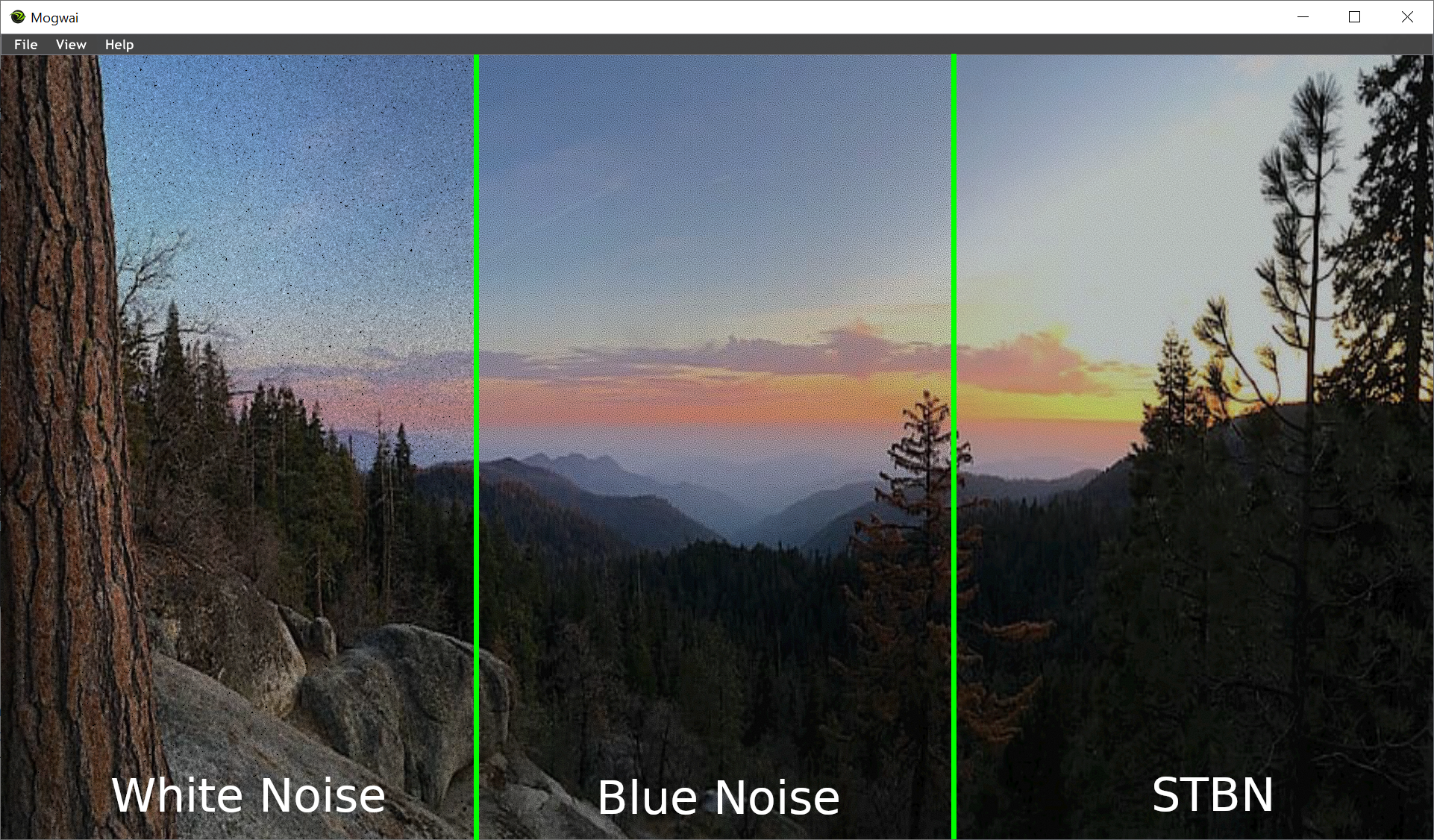
In Figure 3, white noise (left) is very noisy due to clumps and voids that aren’t present in blue noise (center). Our spatiotemporal blue noise does better by having pixels survive evenly not just over space but also over time.

Vectors

Vector spatiotemporal blue noise textures store a vector value per pixel and are useful for rendering algorithms that want a random vector per pixel, such as ray traced ambient occlusion. You generate these textures by running the algorithm from Blue-noise Dithered Sampling (BNDS) in 3D. You make the same modification to the energy function in that paper as you did for scalars in void and cluster. You only return a nonzero energy if they are from the same texture slice, or if they are the same pixel at different points in time. 

The result is again N textures, which are perfectly blue over space, but each pixel individually is also blue over the z axis. Unit vectors can be used, which are useful for situations where you need direction vectors, and nonunit vectors can be used, which are useful when you just need an N dimensional random number, such as a point in space.

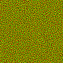
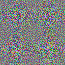
Figure 4 shows slices of vector valued spatiotemporal blue noise, as well as their frequency components over the space and time axis. This shows that they are blue over space and blue over time.

	Vec1	Unit Vec1	Vec2	Unit Vec2	Vec3	Unit Vec3
XY[0]
DFT(XY)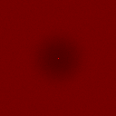
DFT(XZ)

Figure 5 shows 4 sample per pixel ray traced ambient occlusion (AO) using various types of unit vec3 noise. If a vector is facing towards the normal, it is negated. The difference in quality is apparent between white noise, independent blue noise textures, and spatiotemporal blue noise.

Importance sampling

The BNDS algorithm starts with a set of white noise textures and repeatedly swaps pixels at random, if the swap improves the energy function. There is no reason why these textures must be initialized to uniform white noise vectors, though. 

When initializing them to a non-uniform distribution, the algorithm still works in creating blue noise textures. The result is spatiotemporal blue noise textures, which also happen to have a non-uniform histogram, which allows importance sampling. As you need the PDF per pixel to do importance sampling, you can either store the PDF(x) in the alpha channel or calculate the PDF from the value in the texture, such as by doing a dot product if it is cosine hemisphere-weighted or dividing by a normalization value passed in as a shader constant.

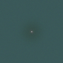
Figure 6 shows importance sampled, vector-valued, spatiotemporal blue noise textures.

	Texture[0]	DFT(XY)	DFT(ZY)	Importance Map
Cosine Weighted Hemisphere Unit Vec3				N/A
HDR Skybox Importance Sampled Unit Vec3

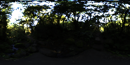Figure 7 shows four-sample per pixel ray traced AO again but using cosine-weighted–hemisphere, importance-sampled unit vectors. White noise makes a unit vec3, adds it to the normal, and normalizes. Blue noise and STBN have cosine-weighted hemispherical vectors stored in their textures, which are transformed into tangent space using a TBN basis matrix.

• Looking at the ovals at the top of the carousel shows how blue noise does better than white noise.
• Looking at the window frames in the upper right, you can see how STBN has less noise in the shadows than independent blue noise textures do.

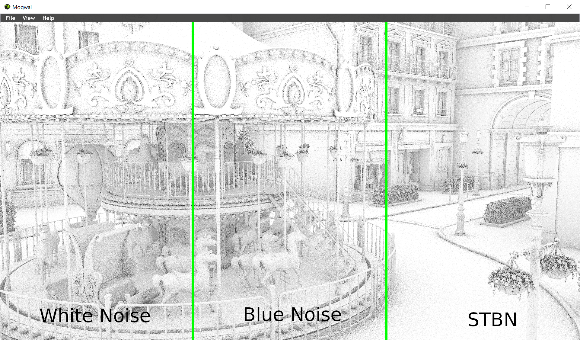
In Figure 7, the difference between the noise is less obvious than when uniform sampling but is still there. The noise in blue noise is harder to see and easier to filter than white noise. The noise in STBN is the same way but is also lower magnitude.

Conclusion

Blue noise can be a great way to get better-looking images at low sample counts, like those found in real-time rendering. Blue noise can be useful in nearly any situation that needs one or more random values per pixel.

Have ideas for using blue noise? Download the textures, give it a try, and share your results in the comments. We’d love to see them!