First responders don’t have time on their side. Whether fires, search-and-rescue missions or medical emergencies, their challenges are usually dangerous and time-sensitive. Using autonomous technology, Zurich-based Fotokite is developing a system to help first responders save lives and increase public safety. Fotokite Sigma is a fully autonomous tethered drone, built with the NVIDIA Jetson platform, Read article >
With the holiday season comes many joys for GeForce NOW members. This month, RTX 3080 membership preorders are activating in Europe. Plus, we’ve made a list — and checked it twice. In total, 20 new games are joining the GeForce NOW library in December. This week, the list of nine games streaming on GFN Thursday Read article >
I have a project in which I will make a model that classifies Knee MRIs from the OAI dataset. My university provided me the dataset.
The classification is about knee osteoartrithis. The model must assign a grade (from 0 to 4) in each MRI.
I am facing a problem as I am not able to find the labels in the MRI file tha was given to me. Is the label somewhere in the metadata or the header of the DICOM files (MRIs) and I cannot find it or my professor forgot to send me an extra file containing the labels ?
In this round of MLPerf training v1.1, optimization across the entire stack including hardware, system software, libraries, and algorithms continue to boost NVIDIA MLPerf training performance.
Five months have passed since v1.0, so it is time for another round of the MLPerf training benchmark. In this v1.1 edition, optimization over the entire hardware and software stack sees continuing improvement across the benchmarking suite for the submissions based on NVIDIA platform. This improvement is observed consistently at all different scales, from single machines all the way to industrial super-computers such as the NVIDIA Selene consisting of 560 NVIDIA DGX A100 systems and the Microsoft Azure NDm A100 v4 cluster consisting of 768-node A100-based systems.
Increasingly, organizations are using the MLPerf benchmarks to guide their AI infrastructure strategies. MLPerf (part of MLCommons) is a global consortium of AI leaders from academia, research labs, and industry whose mission is to build fair and useful benchmarks that provide unbiased evaluations of training and inference performance for hardware, software, and services—all conducted under prescribed conditions. To stay on the cutting edge of industry trends, MLPerf continues to evolve, holding new tests at regular intervals and adding new workloads that represent the state of the art in AI.
As in the previous rounds of the MLPerf benchmark, this post provides a technical deep dive into the optimization work underlying NVIDIA’s industry-leading performance. For more information about previous rounds, see the following posts:
Continuing to disclose and elaborate on these technical details, NVIDIA shows a strong commitment to the important issue of open and fair community-driven benchmarking standards and practices for the advancement of AI for public good.
Optimization across the entire stack
With the building blocks still centered around the now well-established NVIDIA A100 GPU, the NVIDIA DGX A100 platform and the NVIDIA SuperPod reference architecture, optimizations across the entire stack, especially on the system software, libraries and algorithmic fronts, have led to continuing performance improvements of NVIDIA-based platforms in MLPerf v1.1.
Compared to our own MLPerf v0.7 submissions 1 year ago, we observed up to 2.1x improvement on a chip-to-chip basis and up to 5.3x for max-scale training, as shown in Table 1.
Per-Accelerator performance for A100 computed using NVIDIA 8xA100 server time-to-train and multiplying it by 8 (**). U-Net and RNN-T were not part of MLPerf v0.7. MLPerf name and logo are trademarks. For more information, see www.mlperf.org.
The next sections cover some highlights.
CUDA Graphs
In MLPerf v1.0, we extensively used CUDA Graphs for most of the benchmarks. CUDA Graphs launched several kernels as a single executable unit to accelerate throughput by minimizing communication with the CPU. But the scope of each graph was only a portion of one full iteration, which processes a single minibatch. As a result, only part of an iteration was captured as each iteration was broken down into multiple CUDA graphs.
In MLPerf v1.1, we used CUDA Graphs to capture an entire iteration into a single graph for multiple benchmarks, further minimizing communication with the CPU during training and improving the performance at scale. This was implemented for both the PyTorch and MXNet benchmarks, resulting in up to 6% performance gains in the ResNet-50 and BERT workloads.
NCCL
NCCL, part of NVIDIA Magnum IO technologies, is the library that optimizes inter-GPU communication for your server topology. A key feature in NCCL that was added earlier this year was support for CUDA Graphs. This enabled us to capture the entire iteration as a single graph, as described in the previous section.
Previously, NCCL copied all the weights from the graph and performed an all-reduce function, which sums all the weights. The updated weights are then written back to the graph. This required multiple copies of the data.
We have now introduced user buffer registration, where pointers are used by NCCL collectives to avoid copying the data back and forth when used alongside the Scalable Hierarchical Aggregation And Reduction Protocol (SHARP), also part of NVIDIA Magnum IO. In the presence of CUDA Graphs and SHARP, we observed about 2% of end-to-end additional speedup.
NCCL has also implemented fusing scaling ops (multiplying by a scalar) into the communication kernels to reduce data copies, resulting in up to an additional ~3% end-to-end savings in communication-heavy networks like BERT.
Fine-grained overlapping
In this round, we have strongly leveraged the capabilities of GPU hardware that enables the fine-grained overlap of independent computation blocks with each other across multiple cores, as well as increased overlap of communication and computation. This improved the performance, especially of max-scale training, up to 10% on Mask R-CNN and 27% on DLRM.
For the recommender systems benchmark (DLRM) in particular, we made use of the capabilities of software and hardware to use GPU resources efficiently by overlapping multiple operations:
Overlapping embedding index computations with the all-reduce collective of the previous iteration
Overlapping data gradient and weight gradient computations
Increased overlapping of math and other multi-GPU collectives, such as all-to-all
For 3D-UNet, spatial parallelism performance is improved by more efficient scheduling of math and communication kernels for increased overlap of the two.
For Mask R-CNN, we have implemented overlapping of loss computation for mask head, bounding-box head, and RPN-head for improved GPU utilization at scale.
We have significantly improved multi-GPU group batch norm (GBN) performance through more efficient memory copies (vectorization) and better overlap of communication and math within the kernel. This enables scaling the workloads to more GPUs, resulting in more than 10% savings of max-scale training for some computer vision benchmarks such as ResNet50 and SSD and 5% savings for 3D-UNet.
Kernel fusion and optimization
Finally, for the first time in this MLPerf round, we have introduced the fusion of bias gradient reduction into matrix multiplication kernels (fusing of two operations). This results in up to 3% performance improvements.
Model optimization specifics
In this section, we dive into the optimization work on each of the workloads.
BERT
Fusing bias gradient reduction into matrix multiplication in backward pass
The cuBLAS library recently introduced a new type of fusion: fusing bias gradient computation and weight gradient computation in the same kernel.
In this round, we used this cuBLAS feature to fuse these two operations in the backward pass. We also fused bias addition and matrix multiplication in the forward pass. Figure 1 shows the fused operations for the forward pass and backward pass.
Figure 1. Fusing other operations with matrix multiplication in the forward pass (left) and backward pass (right)
Improved fused multihead attention
In the previous round, we implemented fusing of the multihead attention module. This module used parallelism across the num_sequences and num_heads variables. This means that there are a total of num_sequences*num_heads thread blocks that are scheduled simultaneously on different streaming multiprocessors (SMs) on the GPU. num_heads is 16 in the MLPerf BERT model, and when num_sequences is smaller than 6, there are not enough thread blocks to fill the GPU, limiting the parallelism.
In this round, we improved these kernels by introducing slicing across the sequence dimension for batched matrix multiplications required for attention computation, which helped increase the parallelism proportionately. This optimization resulted in an ~8% end-to-end speedup for max-scale training scenarios, where the per-chip batch size is small.
Full iteration graph capture with CUDA Graphs
As mentioned in the previous section on CUDA Graphs, in this round, we captured the full iteration of BERT into a single CUDA graph. This was possible due to CUDA Graphs support in the NCCL communications library, as well as the PyTorch framework. This resulted in ~3% end-to-end savings due to reduced CPU latency and jitter at scale. On top of that, we also leveraged NCCL user-buffer preregistration feature when CUDA Graphs is used, resulting in another ~2% of end-to-end performance improvement.
Setting model parameter buffers to point to a contiguous flat buffer
BERT uses a distributed optimizer to speed up optimization steps. For best all-gather performance, the intermediate buffers used in a distributed optimizer for weight parameters should all be part of a single contiguous flat buffer. This way, instead of running several all-gather functions on small separate tensors, we can better use GPU interconnects by running all-gather for one large message.
On the other hand, PyTorch by default allocates separate buffers for each of the model’s parameter tensors to be used during the forward pass. This requires an extra “unflattening” step, as shown in Figure 2, between the end of an iteration and the beginning of the next one.
In this MLPerf round, we used a single contiguous buffer where each parameter tensor is placed next to each other as part of one big buffer. This removes the need for the extra unflattening step, as shown in Figure 2. This optimization results in ~4% end-to-end performance savings for BERT at max-scale configurations, where the cost of optimizer and parameter copies is most pronounced.
Figure 2.How the parameter tensors are represented in memory between several different steps of an iteration before and after the optimization.
DLRM
HugeCTR, a recommendation system dedicated training framework, part of NVIDIA Merlin, continues to power NVIDIA DLRM submission.
Hybrid embedding index precomputing
In the previous MLPerf round, we implemented hybrid embedding to reduce the communication between GPUs.
Even though the hybrid embedding implemented in HugeCTR significantly reduces the communication traffic, it requires indices to be calculated to determine where to read and distribute the embedding vectors stored on each GPU. The index calculation only relies on the input data, which is prefetched onto the GPU a few iterations ahead. Therefore, in HugeCTR, index precomputing is leveraged as an optimization to hide the cost of computing the indices under the communication kernels of the previous iteration.
Sharing the same spirit as index precomputing in training iterations, the hybrid embedding indices for evaluation can be computed and cached when the evaluation is performed for the first time. They can be reused for the remaining evaluations, which completely removes the cost of computing the indices for subsequent evaluations.
Better overlapping between communication and computation
In DLRM, to facilitate model-parallel training, two all-to-all collectives are needed in the forward and backward phases, respectively. In addition, there is an all-reduce collective at the end of the training for the data-parallel part of the model. How to overlap computation with these communication collectives is key to achieve a high utilization of the GPU, and a high training throughput. A few optimizations have been made to enable a better overlap. Figure 3 shows a simplified timeline for one training iteration.
In the forward propagation phase, the bottom MLP is performed while the forward all-to-all kernel is waiting for the data to arrive. In the backward propagation phase, all-reduce and all-to-all are overlapped to increase the utilization of the network. The index precomputation is also scheduled to overlap with these two communication collectives to use the idle resources on the GPU, maximizing the training throughput.
Figure 3. A simplified timeline view of a training iteration, illustrating fine-grained overlap of compute and communication operations.
Asynchronous weight gradients computing
The data gradient computation and weight gradient computation of an MLP are two independent branches of computations that share the same input. Unlike the data gradients, weight gradients are not needed until the gradient all-reduce. Thanks to the flexibility of the GPU in scheduling kernels, these two computations are performed in parallel in HugeCTR, maximizing the utilization of the GPU.
Better fusions
Kernel fusion is an effective way to reduce trips to memory, improving the GPU utilization. Many fusion patterns have been leveraged in DLRM to achieve better performance previously. For example, the data gradient calculation, ReLU backward operation and bias gradient calculation can be fused together in HugeCTR through cuBLAS. Such a cross-layer fusion pattern leaves the last bias gradient computation unfused.
In this round, the GEMM and bias gradient fusion supported in cuBLAS is leveraged to fuse the bias gradient computation into the weight gradient computation for the last layer of an MLP.
Another fusion example is weight conversion fusion. To support mixed-precision training, the FP32 master weights must be casted into FP16 weights during training. As an optimization, this precision casting is fused with the SGD optimizer in HugeCTR. Whenever an FP32 master weight is updated, it writes out an FP16 version of the updated weight into the memory, eliminating the need for a separate kernel for doing the conversion.
Mask R-CNN
NEEDS LEAD-IN SENTENCE
Using NHWC layout for all the convolutional layers
The ResNet-50 backbone has used the NHWC layout for a long time, but the rest of the model used NCHW up until now.
This round we were able to switch the FPN module (which immediately follows the ResNet-50 backbone) to NHWC. Running FPN in NHWC means we can transpose the outputs instead of the inputs, which is more efficient because the inputs are much larger than the outputs. This change boosted the performance by 4-5% for the max-scale configurations.
Using dedicated nodes exclusively for evaluation for multinode scenario
Although evaluation overlaps with training, Mask R-CNN evaluation is a resource-intensive process. Inevitably, training performance suffers slightly when evaluation is running simultaneously. For max-scale configurations, evaluation takes almost as long as training. Having evaluation constantly running in the background significantly affects the training performance.
One way to overcome this issue is to use a separate set of nodes for evaluation, that is, one set of nodes does training and a smaller set of nodes does evaluation. Implementing this change for max-scale configurations boosted the end-to-end performance by 12%.
Using multithreaded COCO evaluation
The COCO evaluation function consumes most of the evaluation time and is run separately on the bounding box and segmentation mask results. A couple of rounds ago we overlapped these two evaluation calls by running them in multiple processes.
This round, we enabled multi-threaded processing with openmp for the COCO evaluation loop. This is an optional feature in the NVIDIA version of the COCO API software. The evaluation loop can be parallelized by providing an optional argument that specifies the desired number of threads. This optimization improves evaluation speed by about 10%, but only the last evaluation is exposed, so the effect on end-to-end time is much smaller, about 0.5%.
Two-stage top-K computation with quadrupled occupancy for small batch-size runs
We make a couple of top-K calls in Mask R-CNN that take a long time due to low occupancy. The number of cooperative thread arrays, or CTAs (thread blocks) launched by the top-K kernel is proportional to the per-GPU batch size. Max-scale configurations use a per-GPU batch size of 1, which results in only five CTAs being launched. Each CTA is assigned one SM, while the A100 has more than 100 SMs, suggesting low utilization of the GPU.
To alleviate this, we implemented a two-stage approach:
In the first stage, we split the input into four equal parts and then we do top-K on each part with a single call.
In the second stage, we concatenate the four temporary results and take top-K of that.
This yields the same result as before but runs more than 3x faster because we are now launching 20 CTAs instead of 5 in the first stage. Dividing the input further makes the first stage faster, but also makes the second stage slower.
Splitting the input eight ways instead of four means that 40 CTAs are launched instead of 20 in the first stage. The first stage completes in half the time but, unfortunately, the second stage becomes so much slower that overall performance is better with a four-way split. Implementing a four-way split for the max-scale configuration resulted in a 3-4% performance boost.
Overlapping loss computations for mask head, bounding-box head, and RPN-head
Most of the GPU kernels launched by Mask R-CNN suffer from low occupancy when the batch size is small. One way to alleviate this is to overlap execution of as many kernels as possible to take advantage of the GPU resources that would otherwise go idle.
Some of the loss calculations can be done simultaneously. This is true for mask-head loss, bounding-box loss, and RPN-head loss, so we place each of these three loss calculations on different CUDA streams so that they can be executed simultaneously. This boosted the performance by about 5% for max-scale configurations.
3D-UNet
Vectorized concatenate and split operation
3D-UNet uses concatenate operations to concatenate the decoder and encoder activations. This results in device-to-device copies for activation tensors in the forward and backward passes. We optimized these copies by using vectorized loads and stores, doing a 4x wider read/write operation. This speeds up the concat and split operators by over 2.4x, giving an end-to-end speedup of 4.7% on single node configuration and 1.3% on max-scale configuration.
Efficient spatial-parallel convolutions
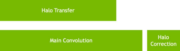
In MLPerf v1.0, we introduced spatial-parallel convolution, where we split the input activation across multiple GPUs (8 to be precise). The implementation of spatial-parallel convolution enabled us to hide the halo exchanges behind convolutions behind the convolution.
In MLPerf v1.1, we optimized the scheduling of communication and convolution operations so that we get a much better overlap between the launched communication and convolution kernels. While this makes sure that the halo exchanges are not exposed, it also helps reduce the jitter significantly. This optimized scheduling improved scores in max-scale configuration by over 25%.
Figure 4. Spatial-parallel convolution: Halo Transfer completely hidden behind convolutions
Spatial-parallel loss calculations
3D-Unet uses the DICE loss and Softmax Cross Entropy loss as its loss functions. The DICE loss is defined as the following formula:
In this formula, and represent pairs of corresponding pixel values of prediction and ground truth, respectively.
In the max-scale configuration, because a single GPU works on just a slice of the image, each GPU holds only a slice of and . To optimize the loss calculation, we calculated the partial terms in each GPU independently and exchanged the partial terms among all the GPUs in the group through NVLink. These partial terms were then combined to form the DICE loss results. This sped up the loss calculation by more than 4x, improving the max-scale score by 7%.
Better configurations
We increased the global batch size to be a factor of dataset size. The DALI data loader library enables us to use the same shard to train for different epochs. This enables us to reduce the time it takes to cache the dataset in the GPU significantly.
Because each GPU loads much fewer images, the Bounding Box cache in DALI warms up much more quickly too. This optimization reduced the startup time significantly and resulted in 20% speedup over MLPerf v1.0.
Data-parallel async evaluation
As training gets faster, scaling evaluation to hide behind training becomes challenging. In MLPerf v1.1, the inferences on a single image were sharded across the GPUs to improve the evaluation scaling. The results of inferences were then all-gathered to form the final output. This enables the entire evaluation phase to be hidden behind training iterations.
Faster group instance norm
The multi-GPU Instancenorm kernel was improved significantly by parallelizing the inter-GPU communication of multiple channel-blocks and reducing the DRAM time of the kernel by vectorizing memory reads and writes. This resulted in throughput improvement of over 5% in the max-scale configuration.
ResNet-50
End-to-end CUDA graphs
For ResNet-50, as the benchmark scales out to >256 nodes, the per-GPU batch size reduces to a very small value, where the iteration time is only ~8-10ms. At these extremely small iteration times, it is critical to ensure there are no gaps in GPU execution arising from dependencies running on the CPU.
For MLPerfV1.1, we reduced jitter at scale by using end-to-end CUDA Graphs to capture an entire iteration across the forward pass, backward pass, optimizer, and Horovord/NCCL gradient all-reduce as a single graph. The use of CUDA Graphs provides a 6% performance benefit at max-scale training.
GBN
As the scale increases for ResNet50 and the local batch sizes decrease, to achieve the fastest possible convergence, we use the GBN technique. For every BatchNorm layer, the mean and variance is all-reduced among a group of GPUs.
For MLPerf v1.1, the performance of GBN within a single DGX node was significantly improved by parallelizing the inter GPU communication of multiple channel-blocks and reducing the DRAM time of the kernel by vectorizing memory reads and writes. This provided a 10% performance benefit at scale.
SSD
On-GPU image caching
Image networks make heavy use of image cropping and resizing to capture features that represent richer statistics of the dataset and to improve the generalization capability of the model.
In the previous MLPerf rounds, SSD used the NVIDIA Data Loading Library (DALI) image decoding features to decode only the cropped region of the JPG image. This feature avoids wasting time decoding the entire image, especially if the crop is small.
However, this means that this cropped image is only used one time as the image is not cached in memory. Future uses of the original image will likely have different cropped regions, meaning that the original image will be decoded each time it is used. This behavior leads to jitter across GPUs as the decoding cost varies greatly on the size of the region required by the crop. This is particularly pronounced for scale-out scenarios.
For this round, we took advantage of the 80-GB memory capacity available to each NVIDIA A100 80-GB GPU by using another DALI feature that decodes the entire image and caches it in memory. This enables future uses of the same image to avoid the decoding cost and instead pick the cropped region directly from memory. Doing this is cheaper than decoding the cropped region each time and has much less run-to-run and device-to-device variation in execution time.
Overall, this optimization resulted in 2% end-to-end performance improvement in our single node configuration and ~5% improvement in our efficient-scale configuration, which is in between single-node and max-scale in terms of scale.
GBN for SSD
SSD also took advantage of the GBN improvements implemented in ResNet-50, which gave a ~4% E2E improvement in our max-scale configuration.
RNN-T
More optimized apex transducer
The transducer module in apex has been further optimized to improve the training throughput. Two optimizations have been added to the transducer joint and transducer loss module, respectively.
Transducer joint, ReLU, and dropout are three consecutive memory-bound operations in RNN-T. As an optimization, ReLU and dropout have been fused with the transducer joint in the apex.contrib.transducer.TransducerJoint module in apex, effectively cutting the trips to the memory.
The backward propagation of the transducer loss is a memory-intensive operation. An optimization of vectorizing the loads and stores in the backward operation has been added to apex.contrib.transducer.TransducerLoss in apex, improving the memory bandwidth utilization of the kernel.
More data preprocessing on GPU
Preprocessing the next batch on the CPU while the GPU is busy with a forward and backward pass can hide data preprocessing time. This is ideal. However, when data preprocessing is compute-intensive, the preprocessing time on the CPU might get exposed.
DALI can help unload the CPU by computing parts of the preprocessing on GPU, leveraging the massively parallel processing nature of the GPU. In this submission, the silence trimming operation was moved to GPU, improving the training throughput.
Conclusion
Building upon the well-established and proven NVIDIA A100 GPU and NVIDIA DGX A100 platforms, optimization across the stacks continues to deliver performance improvements across the board for NVIDIA platform-based submissions in this round of MLPerf v1.1 training benchmark.
It is worth reiterating that the NVIDIA platform has been the only solution to make submissions across all workloads in the MLPerf benchmarking suite, demonstrating both industry-leading performance and versatility.
All software used for NVIDIA submissions is available from the MLPerf repository, to enable you to reproduce our benchmark results. We constantly add these cutting-edge MLPerf improvements into our deep learning frameworks containers available on NGC, our software hub for GPU-optimized applications.
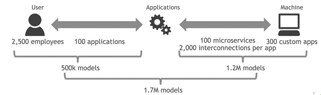
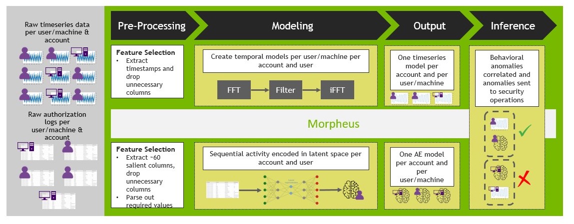
Use unsupervised AI and time series modeling to create microtargeted models for every user and account; as humans and machine/account combinations running on your network.
Traditional approaches to finding and stopping threats have ceased to be appropriately effective. One reason is the scope of ways an attacker can enter a system and do damage have proliferated as the interconnections between apps and systems have proliferated.
Applying AI to the problem seems like a natural choice but this in some sense broadens the data problem. A typical user may interact with 100 or more apps while doing their job, and integrations between apps means that there may be tens of thousands of interconnections and permissions shared across those 100 apps. If you have 10,000 users, you’d need 10,000 models as a beginning.
The good news is that NVIDIA Morpheus addresses this problem. NVIDIA recently announced an update to Morpheus, an end-to-end tool to apply data science to cybersecurity problems.
While most apps and systems will create logs, the variety, volume, and velocity of these logs means that much of the response possible is “closing the barn door after the horse has left.” Identifying credential breaches and the damage done can take weeks if you’re lucky, months if you’re average.
With any number of users beyond “modest” or “very modest,” traditional rule-based systems to create warnings are insufficient. A person who knew how another person or system typically behaves could notice something fishy almost immediately when that user or system started doing something that was unusual.
Every account has a digital fingerprint: a typical set of things it does or doesn’t do in a specific sequence in time. This problem is no longer addressed by just strong passwords that reset periodically, a table of rules, and periodic drop-sized spot checks of logs from the ocean of log data.
The problem is understanding every user’s day-to-day, moment-by-moment work. This is a data science problem.
Model ensemble for multiple methods
10,000 models are daunting enough. But if we’re committed to approaching the cybersecurity problem like the serious data science problem it is, one model isn’t enough. The state of the art in the most critical data-science problems is ensembling multiple models.
A model ensemble is where models are combined in some way to give better predictions than a single model could. The “wisdom of the crowd” turns out to be just as true, with a crowd of machine learning methods all trying to predict the same thing.
In the case of identifying the digital fingerprint of a malevolent attack, Morpheus takes two different models and uses them to alert human analysts to possible serious danger. One method is only a few years old and the other is several hundred years old:
Because attacks seek to hide their behavior by mimicking a given account’s behavior, autoencoders test how typical a given user’s behavior is as a flat snapshot.
Because an attack is temporal, Fourier transforms are used to understand the typical behavior over time.
Method 1: Autoencoders
In the specific example that is enabled with Morpheus, an autoencoder is trained on AWS CloudTrail data. The CloudTrail logs are nested JSON objects that can be transformed into tabular data. The data fields can vary widely across time and users. This requires the flexibility that neural net methods provide and the preprocessing speed of RAPIDS, a part of the Morpheus platform. The particular neural net method that Morpheus deploys in this use case is an autoencoder.
At a high level, an autoencoder is a type of neural network that tries to extract noise from a given datum and reconstruct that datum in an approximated form without that noise while being as true as possible to the actual datum.
For example, think of a photograph with scratches over the surface. A good autoencoder reproduces the underlying picture without the scratches. A well-trained autoencoder, one that knows its domain well, has low “loss” or error as it reconstructs a given datum.
In this case, you take a given user’s typical behavior, take out the “noise” of slight variation, and reproduce that digital fingerprint. Each encoding event has a loss or error associated with it, like any statistics problem.
To deploy this solution, update the pretrained model that comes with Morpheus with a period of typical, attack-free data for each user/service and machine/service interaction. Move these models to the NVIDIA Triton Inference Server layer of Morpheus.
What may be surprising is that the actual auto-encoding is discarded and the loss number is preserved. A user-defined threshold is defined to flag accounts to be reviewed by a human. The default option is a classic Z-score: Is the loss four standard deviations higher than the average loss for this user?
Figure 2. The combinatorial explosion of the modern enterprise and its security requirements
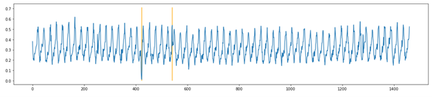
Method 2: Fast Fourier Transforms
Figure 3. Two timepoints of anomalous activity captured by the Morpheus framework that likely would go undetected without time series analysis like FFT
Fast Fourier transforms (FFTs) distill the essential behavior of a wave under the data noise. Fourier analysis was developed in the late 1700s and has continued to be invaluable to the applied mathematical analysis of fields as diverse as finance, traffic engineering, economics, and in this case, cybersecurity.
A given time series is compostable into various components, showing regular seasonal, weekly, and hourly variations along with a trend. Decomposing a time series enables analysts to understand if something that goes up and down a lot over time is actually growing despite constant oscillations. They can also understand if the time series is of interest to the cybersecurity use case, and if there is something truly unusual going on beyond the normal ebb and flow of traffic.
Machine application activity tends to oscillate over time, and attacker activities can be difficult to detect among the periodic noise in data with just a volumetric alert. To find subtle anomalies inside periodic data, you transform the data from the time domain to the frequency domain using FFT. You then reconstruct the signal back to the time domain (with iFFT) but use only the top 90% of frequencies. A large difference between the original signal and the reconstructed signal indicates the times at which the machine’s activity is unusual and potentially compromised by malicious human activity.
Morpheus applies FFTs by learning what a normal period or periods of activity looks like for a given user/service and machine/service system interaction. After this, GPUs perform decomposition quickly and apply a rolling Z-score to the transformed data to flag periods that are anomalous. For reference, CuPy FFT decompositions are as much as 120x faster than comparable operations done through NumPy. For more information, see FFT Speedtest comparing Tensorflow, PyTorch, CuPy, PyFFTW and NumPy.
Putting it all together
Morpheus is a tool to aid human analysts. This means that it is at its most useful when it sends the right amount of data to a person.
Figure 4. NVIDIA Morpheus workflow
Returning to the ensembling discussion from earlier, Morpheus uses a voting ensemble. Data flagged by both models with the most urgency is sent to the human security team. This enables a force multiplier for cybersecurity red teams by directing their valuable time to threats as they unfold in real time, rather than weeks or months later.
The cybersecurity data problem is like refining ore from silt: you begin with a huge amount of nothing and as you sift, refine, and assay, you get to something actually worth looking at. While we wouldn’t suggest that system intrusions are gold, we know that the time of analysts is.
Effective defense requires intelligence tools to aid traceability and prioritization. The ensembling of sophisticated methods that Morpheus deploys does just that. This means reduced financial, reputational, and operational risk for enterprises that deploy Morpheus.
Try it out
Morpheus ships with the code, data, and models for you to be able to see how the use case works and to get a feel for how Morpheus would work for your enterprise. Using the earlier workflow, you observed a micro-F1 score of 1. In addition, across multiple experiments, you saw a near 0% rate of false attribution (machine compared to human).
Beyond the state-of-the-art data science and prebuilt models, Morpheus is designed to be a platform for cybersecurity data science. It seamlessly combines a suite of NVIDIA and Cyber Log Accelerator (CLX) technologies to make deployment easy and fast.
Keep in mind that these models, particularly the FFT model, cannot start totally cold and must be given some amount of data that is representative of a normal, attack-free stream of CloudTrail logs.
This is just the beginning of what Morpheus can do to stop the hacking specter haunting enterprises. It is easy to imagine that, in the near future, even more models are deployed simultaneously for even greater predictive accuracy. For access to the latest release of NVIDIA Morpheus, register for the expanded early access program.
Posted by Sabela Ramos, Software Engineer and Léonard Hussenot, Student Researcher, Google Research, Brain Team
Most reinforcement learning (RL) and sequential decision making algorithms require an agent to generate training data through large amounts of interactions with their environment to achieve optimal performance. This is highly inefficient, especially when generating those interactions is difficult, such as collecting data with a real robot or by interacting with a human expert. This issue can be mitigated by reusing external sources of knowledge, for example, the RL Unplugged Atari dataset, which includes data of a synthetic agent playing Atari games.
However, there are very few of these datasets and a variety of tasks and ways of generating data in sequential decision making (e.g., expert data or noisy demonstrations, human or synthetic interactions, etc.), making it unrealistic and not even desirable for the whole community to work on a small number of representative datasets because these will never be representative enough. Moreover, some of these datasets are released in a form that only works with certain algorithms, which prevents researchers from reusing this data. For example, rather than including the sequence of interactions with the environment, some datasets provide a set of random interactions, making it impossible to reconstruct the temporal relation between them, while others are released in slightly different formats, which can introduce subtle bugs that are very difficult to identify.
In this context, we introduce Reinforcement Learning Datasets (RLDS), and release a suite of tools for recording, replaying, manipulating, annotating and sharing data for sequential decision making, including offline RL, learning from demonstrations, or imitation learning. RLDS makes it easy to share datasets without any loss of information (e.g., keeping the sequence of interactions instead of randomizing them) and to be agnostic to the underlying original format, enabling users to quickly test new algorithms on a wider range of tasks. Additionally, RLDS provides tools for collecting data generated by either synthetic agents (EnvLogger) or humans (RLDS Creator), as well as for inspecting and manipulating the collected data. Ultimately, integration with TensorFlow Datasets (TFDS) facilitates the sharing of RL datasets with the research community.
With RLDS, users can record interactions between an agent and an environment in a lossless and standard format. Then, they can use and transform this data to feed different RL or Sequential Decision Making algorithms, or to perform data analysis.
Dataset Structure Algorithms in RL, offline RL, or imitation learning may consume data in very different formats, and, if the format of the dataset is unclear, it’s easy to introduce bugs caused by misinterpretations of the underlying data. RLDS makes the data format explicit by defining the contents and the meaning of each of the fields of the dataset, and provides tools to re-align and transform this data to fit the format required by any algorithm implementation. In order to define the data format, RLDS takes advantage of the inherently standard structure of RL datasets — i.e., sequences (episodes) of interactions (steps) between agents and environments, where agents can be, for example, rule-based/automation controllers, formal planners, humans, animals, or a combination of these. Each of these steps contains the current observation, the action applied to the current observation, the reward obtained as a result of applying action, and the discount obtained together with reward. Steps also include additional information to indicate whether the step is the first or last of the episode, or if the observation corresponds to a terminal state. Each step and episode may also contain custom metadata that can be used to store environment-related or model-related data.
Producing the Data Researchers produce datasets by recording the interactions with an environment made by any kind of agent. To maintain its usefulness, raw data is ideally stored in a lossless format by recording all the information that is produced, keeping the temporal relation between the data items (e.g., ordering of steps and episodes), and without making any assumption on how the dataset is going to be used in the future. For this, we release EnvLogger, a software library to log agent-environment interactions in an open format.
EnvLogger is an environment wrapper that records agent–environment interactions and saves them in long-term storage. Although EnvLogger is seamlessly integrated in the RLDS ecosystem, we designed it to be usable as a stand-alone library for greater modularity.
As in most machine learning settings, collecting human data for RL is a time consuming and labor intensive process. The common approach to address this is to use crowd-sourcing, which requires user-friendly access to environments that may be difficult to scale to large numbers of participants. Within the RLDS ecosystem, we release a web-based tool called RLDS Creator, which provides a universal interface to any human-controllable environment through a browser. Users can interact with the environments, e.g., play the Atari games online, and the interactions are recorded and stored such that they can be loaded back later using RLDS for analysis or to train agents.
Sharing the Data Datasets are often onerous to produce, and sharing with the wider research community not only enables reproducibility of former experiments, but also accelerates research as it makes it easier to run and validate new algorithms on a range of scenarios. For that purpose, RLDS is integrated with TensorFlow Datasets (TFDS), an existing library for sharing datasets within the machine learning community. Once a dataset is part of TFDS, it is indexed in the global TFDS catalog, making it accessible to any researcher by using tfds.load(name_of_dataset), which loads the data either in Tensorflow or in Numpy formats.
TFDS is independent of the underlying format of the original dataset, so any existing dataset with RLDS-compatible format can be used with RLDS, even if it was not originally generated with EnvLogger or RLDS Creator. Also, with TFDS, users keep ownership and full control over their data and all datasets include a citation to credit the dataset authors.
Consuming the Data Researchers can use the datasets in order to analyze, visualize or train a variety of machine learning algorithms, which, as noted above, may consume data in different formats than how it has been stored. For example, some algorithms, like R2D2 or R2D3, consume full episodes; others, like Behavioral Cloning or ValueDice, consume batches of randomized steps. To enable this, RLDS provides a library of transformations for RL scenarios. These transformations have been optimized, taking into account the nested structure of the RL datasets, and they include auto-batching to accelerate some of these operations. Using those optimized transformations, RLDS users have full flexibility to easily implement some high level functionalities, and the pipelines developed are reusable across RLDS datasets. Example transformations include statistics across the full dataset for selected step fields (or sub-fields) or flexible batching respecting episode boundaries. You can explore the existing transformations in this tutorial and see more complex real examples in this Colab.
Available Datasets At the moment, the following datasets (compatible with RLDS) are in TFDS:
three Robosuite datasets generated with the RLDS tools
Our team is committed to quickly expanding this list in the near future and external contributions of new datasets to RLDS and TFDS are welcomed.
Conclusion The RLDS ecosystem not only improves reproducibility of research in RL and sequential decision making problems, but also enables new research by making it easier to share and reuse data. We hope the capabilities offered by RLDS will initiate a trend of releasing structured RL datasets, holding all the information and covering a wider range of agents and tasks.
Acknowledgements Besides the authors of this post, this work has been done by Google Research teams in Paris and Zurich in Collaboration with Deepmind. In particular by Sertan Girgin, Damien Vincent, Hanna Yakubovich, Daniel Kenji Toyama, Anita Gergely, Piotr Stanczyk, Raphaël Marinier, Jeremiah Harmsen, Olivier Pietquin and Nikola Momchev. We also want to thank the collaboration of other engineers and researchers who provided feedback and contributed to the project. In particular, George Tucker, Sergio Gomez, Jerry Li, Caglar Gulcehre, Pierre Ruyssen, Etienne Pot, Anton Raichuk, Gabriel Dulac-Arnold, Nino Vieillard, Matthieu Geist, Alexandra Faust, Eugene Brevdo, Tom Granger, Zhitao Gong, Toby Boyd and Tom Small.
Leonardo da Vinci’s portrait of Jesus, known as Salvator Mundi, was sold at a British auction for nearly half a billion dollars in 2017, making it the most expensive painting ever to change hands. However, even art history experts were skeptical about whether the work was an original of the master rather than one of Read article >
Look who just set new speed records for training AI models fast: Dell Technologies, Inspur, Supermicro and — in its debut on the MLPerf benchmarks — Azure, all using NVIDIA AI. Our platform set records across all eight popular workloads in the MLPerf training 1.1 results announced today. NVIDIA A100 Tensor Core GPUs delivered the Read article >
The NVIDIA Network Operator includes an RDMA Shared Device Plug-In and OFED Driver.
The NVIDIA GPU Operator has NVIDIA GPU Monitoring, NVIDIA Container Runtime, NVIDIA Driver, and NVIDIA Kubernetes Device Plug-In.
When deployed together, they automatically enable the GPU Direct RDMA Driver.
The NVIDIA EGX Operators are part of the NVIDIA EGX stack which contain Kubernetes, Container engine and Linux Distribution. They run bare metal virtualization.
Installing the Network Operator with a custom driver container
Installing the GPU Operator with a custom driver container
NVIDIA Driver integration
The preinstalled driver integration method is suitable for edge deployments requiring signed drivers for secure and measured boot. Use the driver container method when the edge node has an immutable operating system. Driver containers are also appropriate when not all edge nodes have accelerators.
Clean up preinstalled driver integration
First, uninstall the previous configuration and reboot to clear the preinstalled drivers.
Delete the test pods and network attachment.
$ kubectl delete pod roce-shared-pod
pod "roce-shared-pod" deleted

$ kubectl delete macvlannetwork  roce-shared-macvlan-network
macvlannetwork.mellanox.com "roce-shared-macvlan-network" deleted
3. Uninstall MOFED to remove the preinstalled drivers and libraries.
$ rmmod nvidia_peermem

$ /etc/init.d/openibd stop
Unloading HCA driver:                                      [  OK  ]

$ cd ~/MLNX_OFED_LINUX-5.4-1.0.3.0-rhel7.9-x86_64

$ ./uninstall.sh
4. Remove the GPU test pod.
$ kubectl delete pod cuda-vectoradd
pod "cuda-vectoradd" deleted
5. Uninstall the NVIDIA Linux driver.
$ ./NVIDIA-Linux-x86_64-470.57.02.run --uninstall
6. Remove GPU Operator.
$ helm uninstall gpu-operator-1634173044
7. Reboot.
$ sudo shutdown -r now
Install the Network Operator with a custom driver container
This section describes the steps for installing the Network Operator with a custom driver container.
The driver build script executed in the container image needs access to kernel development and packages for the target kernel. In this example the kernel development packages are provided through an Apache web server.
Once the container is built, upload it to a repository the Network Operator Helm chart can access from the host.
The GPU Operator will use the same web server to build the custom GPU Operator driver container in the next section.
Install the Apache web server and start it.
$ sudo firewall-cmd --state
not running

$ sudo yum install createrepo yum-utils httpd -y

$ systemctl start httpd.service && systemctl enable httpd.service && systemctl status httpd.service
● httpd.service - The Apache HTTP Server
   Loaded: loaded (/usr/lib/systemd/system/httpd.service; enabled; vendor preset: disabled)
   Active: active (running) since Wed 2021-10-20 18:10:43 EDT; 4h 45min ago
...
Create a mirror of the upstream CentOS 7 Base package repository. It could take ten minutes or more to download all the CentOS Base packages to the web server. Note that the custom package repository requires 500 GB free space on the /var partition.
3. Copy the Linux kernel source files into the Base packages directory on the web server. This example assumes the custom kernel was compiled as an RPM using rpmbuild.
$ cd repos/centos/7/x86_64/os
$ sudo cp ~/rpmbuild/RPMS/x86_64/*.rpm .
The Network Operator requires the following files:
kernel-headers-${KERNEL_VERSION}
kernel-devel-${KERNEL_VERSION}
Ensure the presence of these additional files for the GPU Operator:
gcc-${GCC_VERSION}
elfutils-libelf.x86_64
elfutils-libelf-devel.x86_64
$ for i in $(rpm -q kernel-headers kernel-devel elfutils-libelf elfutils-libelf-devel gcc | grep -v "not installed"); do ls $i*; done
kernel-headers-3.10.0-1160.42.2.el7.custom.x86_64.rpm
kernel-devel-3.10.0-1160.42.2.el7.custom.x86_64.rpm
elfutils-libelf-0.176-5.el7.x86_64.rpm
elfutils-libelf-devel-0.176-5.el7.x86_64.rpm
gcc-4.8.5-44.el7.x86_64.rpm
4. Browse to the web repository to make sure it is accessible via HTTP.
5. MOFED driver container images are built from source code in the mellanox/ofed-docker repository on Github. Clone the ofed-docker repository.
$ git clone https://github.com/Mellanox/ofed-docker.git
$ cd ofed-docker/
6. Make a build directory for the custom driver container.
$ mkdir centos
$ cd centos/
7. Create a Dockerfile that installs the MOFED dependencies and source archive into a CentOS 7.9 base image. Specify the MOFED and CentOS versions.
$ sudo cat
8. Modify the RHEL entrypoint.sh script included in the ofed-docker repository to install the custom kernel source packages from the web server. Specify the path to the base/Packages directory on the web server in the _install_prerequsities() function.
In this example 10.150.168.20 is the web server IP address created earlier in the section.
$ cp ../rhel/entrypoint.sh .
$ cat entrypoint.sh
...
# Install the kernel modules header/builtin/order files and generate the kernel version string.
_install_prerequisites() {

    echo "Installing dependencies"
    yum -y --releasever=7 install createrepo elfutils-libelf-devel kernel-rpm-macros numactl-libs initscripts grubby linux-firmware libtool

    echo "Installing Linux kernel headers..."
    rpm -ivh http://10.150.168.20/repos/centos/7/x86_64/os/base/Packages/kernel-3.10.0-1160.45.1.el7.custom.x86_64.rpm
    rpm -ivh http://10.150.168.20/repos/centos/7/x86_64/os/base/Packages/kernel-devel-3.10.0-1160.45.1.el7.custom.x86_64.rpm
    rpm -ivh http://10.150.168.20/repos/centos/7/x86_64/os/base/Packages/kernel-headers-3.10.0-1160.45.1.el7.custom.x86_64.rpm

    # Prevent depmod from giving a WARNING about missing files
    touch /lib/modules/${KVER}/modules.order
    touch /lib/modules/${KVER}/modules.builtin

    depmod ${KVER}
...
9. The OFED driver container mounts a directory from the host file system for sharing driver files. Create the directory.
$ mkdir -p /run/mellanox/drivers
10. Upload the new CentOS driver image to a registry. This example uses an NGC private registry. Login to the registry.
13. Override the values.yaml file included in the NVIDIA Network Operator Helm chart to install the custom driver image. Specify the image name, repository, and version for the custom driver container.
$ cat
14. Install the NVIDIA Network Operator with the new values.yaml.
15. View the pods deployed by the Network Operator. The MOFED pod should be in status Running. This is the custom driver container. Note that it may take several minutes to compile the drivers before starting the pod.
$ kubectl -n nvidia-network-operator-resources get pods
NAME                      READY   STATUS    RESTARTS   AGE
cni-plugins-ds-zr9kf      1/1     Running   0          10m
kube-multus-ds-w57rz      1/1     Running   0          10m
mofed-centos7-ds-cbs74    1/1     Running   0          10m
rdma-shared-dp-ds-ch8m2   1/1     Running   0          2m27s
whereabouts-z947f         1/1     Running   0          10m
16. Verify that the MOFED drivers are loaded on the host.
17. The root filesystem of the driver container should be bind mounted to the /run/mellanox/drivers directory on the host.
$ ls /run/mellanox/drivers
anaconda-post.log  bin  boot  dev  etc  home  host  lib  lib64  media  mnt  opt  proc  root  run  sbin  srv  sys  tmp  usr  var
Install the GPU Operator with a custom driver container
This section describes the steps for installing the GPU Operator with a custom driver container.
Like the Network Operator, the driver build script executed by the GPU Operator container needs access to development packages for the target kernel.
This example uses the same web server that delivered development packages to the Network Operator in the previous section.
Once the container is built, upload it to a repository the GPU Operator Helm chart can access from the host. Like the Network Operator example, the GPU Operator also uses the private registry on NGC.
Build a custom driver container.
$ cd ~
$ git clone https://gitlab.com/nvidia/container-images/driver.git
$ cd driver/centos7
2. Update the CentOS Dockerfile to use driver version 470.74. Comment out unused arguments.
5. Verify that the following files are available in the custom repository created for the Network Operator installation:
elfutils-libelf.x86_64
elfutils-libelf-devel.x86_64
kernel-headers-${KERNEL_VERSION}
kernel-devel-${KERNEL_VERSION}
gcc-${GCC_VERSION}
These files are needed to compile the driver for the custom kernel image.
$ cd /var/www/html/repos/centos/7/x86_64/os/base/Packages/

$ for i in $(rpm -q kernel-headers kernel-devel elfutils-libelf elfutils-libelf-devel gcc | grep -v "not installed"); do ls $i*; done
kernel-headers-3.10.0-1160.45.1.el7.custom.x86_64.rpm
kernel-devel-3.10.0-1160.45.1.el7.custom.x86_64.rpm
elfutils-libelf-0.176-5.el7.x86_64.rpm
elfutils-libelf-devel-0.176-5.el7.x86_64.rpm
gcc-4.8.5-44.el7.x86_64.rpm
6. Unlike the Network Operator, the GPU Operator uses a custom Yum repository configuration file. Create a Yum repo file referencing the custom mirror repository.
$ cd /var/www/html/repos

$ cat
7. The GPU Operator uses a Kubernetes ConfigMap to configure the custom repository. The ConfigMap must be available in the gpu-operator-resources namespace. Create the namespace and the ConfigMap.
$ kubectl create ns gpu-operator-resources

$ kubectl create configmap repo-config -n gpu-operator-resources --from-file=/var/www/html/repos/custom-repo.repo
configmap/repo-config created

$ kubectl describe cm -n gpu-operator-resources repo-config
Name:         repo-config
Namespace:    gpu-operator-resources
Labels:
Annotations:

Data
====
custom-repo.repo:
----
[base]
name=CentOS Linux $releasever - Base
baseurl=http://10.150.168.20/repos/centos/$releasever/$basearch/os/base/
gpgcheck=0
enabled=1
8. Install the GPU Operator Helm chart. Specify the custom repository location, the custom driver version, and the custom driver image name and location.
Defaulted container "nvidia-driver-ctr" out of: nvidia-driver-ctr, k8s-driver-manager (init)
Thu Oct 28 02:37:50 2021
+-----------------------------------------------------------------------------+
| NVIDIA-SMI 470.74       Driver Version: 470.74       CUDA Version: 11.4     |
|-------------------------------+----------------------+----------------------+
| GPU  Name        Persistence-M| Bus-Id        Disp.A | Volatile Uncorr. ECC |
| Fan  Temp  Perf  Pwr:Usage/Cap|         Memory-Usage | GPU-Util  Compute M. |
|                               |                      |               MIG M. |
|===============================+======================+======================|
|   0  NVIDIA A100-PCI...  On   | 00000000:23:00.0 Off |                    0 |
| N/A   25C    P0    32W / 250W |      0MiB / 40536MiB |      0%      Default |
|                               |                      |             Disabled |
+-------------------------------+----------------------+----------------------+
|   1  NVIDIA A100-PCI...  On   | 00000000:E6:00.0 Off |                    0 |
| N/A   27C    P0    32W / 250W |      0MiB / 40536MiB |      0%      Default |
|                               |                      |             Disabled |
+-------------------------------+----------------------+----------------------+

+-----------------------------------------------------------------------------+
| Processes:                                                                  |
|  GPU   GI   CI        PID   Type   Process name                  GPU Memory |
|        ID   ID                                                   Usage      |
|=============================================================================|
|  No running processes found                                                 |
+-----------------------------------------------------------------------------+
The NVIDIA peer memory driver that enables GPUDirect RDMA is not built automatically.
Repeat this process to build a custom nvidia-peermem driver container.
This additional step is needed for any Linux operating system that the nvidia-peermem installer in GPU Operator does not yet support.
The future with NVIDIA Accelerators
NVIDIA accelerators help future-proof an edge AI investment against the exponential growth of sensor data. NVIDIA operators are cloud native software that streamline accelerator deployment and management on Kubernetes. The operators support popular Kubernetes platforms out of the box and can be customized to support alternative platforms.
Recently, NVIDIA announced converged accelerators that combine DPU and GPU capability onto a single PCI device. The converged accelerators are ideal for edge AI applications with demanding compute and network performance requirements. The NVIDIA operators are being enhanced to facilitate converged accelerator deployment on Kubernetes.
Both the NVIDIA GPU Operator and Network Operator are open source software projects published under the Apache 2.0 license. NVIDIA welcomes upstream participation for both projects.
Register for GTC 2021 session, Exploring Cloud-native Edge AI, to learn more about accelerating edge AI with NVIDIA GPUs and SmartNICs.


 In this round of MLPerf training v1.1, optimization across the entire stack including hardware, system software, libraries, and algorithms continue to boost NVIDIA MLPerf training performance.
 and
and  represent pairs of corresponding pixel values of prediction and ground truth, respectively.
 Use unsupervised AI and time series modeling to create microtargeted models for every user and account; as humans and machine/account combinations running on your network.
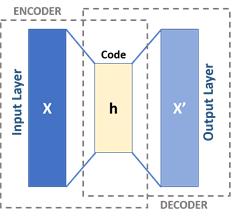

 The NVIDIA Network Operator includes an RDMA Shared Device Plug-In and OFED Driver.