Hello! I’m a long time developer but new to AI-based image processing. The end goal is to process images from cameras and alert when deer (and eventually other wildlife) is detected.
The first step is finding a decent model that can (say) detect deer vs. birds vs. other animals, then running that somewhere. The default The CameraTraps model here allows detecting “animal” vs. “person” vs. “vehicle”:
Would I need to train it further to differentiate between types of animals, or am I missing something with the default model? Or a more general question, how can you see what a frozen model is set up to detect? (I just learned what a frozen model was yesterday)
Appreciate any pointers or if there’s another sub that would be more suited to getting this project setup, happy to post there instead 🙂
Explore NVIDIA Metropolis partners showcasing new technologies to improve city mobility at the ITS America 2021.
The Intelligent Transportation Society (ITS) of America annual conference brings together a community of intelligent transportation professionals to network, educate others about emerging technologies, and demonstrate innovative products driving the future of efficient and safe transportation.
As cities and DOT teams struggle with constrained roadway infrastructure and the need to build safer roads, events like this offer solutions and reveal a peek into the future. The NVIDIA Metropolis video analytics platform is increasingly being used by cities, DOTs, tollways, and developers to help measure, automate, and vastly improve the efficiency and safety of roadways around the world.
The following NVIDIA Metropolis partners are participating at ITS-America and showcasing how they help cities improve livability and safety.
Miovision: Arguably one of the first in building superhuman levels of computer vision into intersections, Miovison will explain how their technology is transforming traffic intersections, giving cities and towns more effective tools to manage traffic congestion, improving traffic safety, and reducing the impact of traffic on greenhouse gas emissions. Check out Miovision at booth #1619.
NoTraffic: NoTraffic’s real-time, plug-and-play autonomous traffic management platform uses AI and cloud computing to reinvent how cities run their transport networks. The NoTraffic platform is an end-to-end hardware and software solution installed at intersections, transforming roadways to optimize traffic flows and reduce accidents. Check out NoTraffic at booth #1001.
Ouster: Cities are using Ouster digital lidar solutions capable of capturing the environment in minute detail and detecting vehicles, vulnerable road users, and traffic incidents in real time to improve safety and traffic efficiency. Ouster lidar’s 3D spatial awareness and 24/7 performance combine the high-resolution imagery of cameras with the all-weather reliability of radar. Check out Ouster and a live demo at booth #2012.
Parsons: Parsons is a leading technology firm driving the future of smart infrastructure. Parsons develops advanced traffic management systems that cities use to improve safety, mobility, and livability. Check out Parsons at booth #1818.
Velodyne Lidar: Velodyne’s lidar-based Intelligent Infrastructure Solution (IIS) is a complete end-to-end Smart City solution. IIS creates a real-time 3D map of roads and intersections, providing precise traffic and pedestrian safety analytics, road user classification, and smart signal actuation. The solution is deployed in the US, Canada and across EMEA and APAC. Learn more about Velodyne’s on-the-ground deployments at their panel talk.
Register for ITS America, happening December 7-10 in Charlotte, NC.
Learn about the latest updates to NVIDIA TAO, an AI-model-adaptation framework, and NVIDIA TAO toolkit, a CLI and Jupyter notebook-based version of TAO.
All AI applications are powered by models. Models can help spot defects in parts, detect the early onset of disease, translate languages, and much more. But building custom models for a specific use requires mountains of data and an army of data scientists.
NVIDIA TAO, an AI-model-adaptation framework, simplifies and accelerates the creation of AI models. By fine-tuning state-of-the-art, pretrained models, you can create custom, production-ready computer vision and conversational AI models. This can be done in hours rather than months, eliminating the need for large training data or AI expertise.
The latest version of the TAO toolkit is now available for download. The TAO toolkit, a CLI and Jupyter notebook-based version of TAO, brings together several new capabilities to help you speed up your model creation process.
Increased utilization of GPUs for faster, more efficient training.
We are also taking TAO to the next level and making it a lot easier to create custom, production-ready models. A graphical user interface version of TAO is currently under development that epitomizes a zero-code model development solution. This creates the ability to train, adapt, and optimize computer vision and conversational AI models without writing a single line of code.
Early access is slated for early 2022. Sign up today!
Posted by Jason Wei, AI Resident and Dan Garrette, Research Scientist, Google Research
In recent years, pre-trained language models, such as BERT and GPT-3, have seen widespread use in natural language processing (NLP). By training on large volumes of text, language models acquire broad knowledge about the world, achieving strong performance on various NLP benchmarks. These models, however, are often opaque in that it may not be clear why they perform so well, which limits further hypothesis-driven improvement of the models. Hence, a new line of scientific inquiry has arisen: what linguistic knowledge is contained in these models?
While there are many types of linguistic knowledge that one may want to investigate, a topic that provides a strong basis for analysis is the subject–verb agreement grammar rule in English, which requires that the grammatical number of a verb agree with that of the subject. For example, the sentence “The dogs run.” is grammatical because “dogs” and “run” are both plural, but “The dogs runs.” is ungrammatical because “runs” is a singular verb.
One framework for assessing the linguistic knowledge of a language model is targeted syntactic evaluation (TSE), in which minimally different pairs of sentences, one grammatical and one ungrammatical, are shown to a model, and the model must determine which one is grammatical. TSE can be used to test knowledge of the English subject–verb agreement rule by having the model judge between two versions of the same sentence: one where a particular verb is written in its singular form, and the other in which the verb is written in its plural form.
With the above context, in “Frequency Effects on Syntactic Rule-Learning in Transformers”, published at EMNLP 2021, we investigated how a BERT model’s ability to correctly apply the English subject–verb agreement rule is affected by the number of times the words are seen by the model during pre-training. To test specific conditions, we pre-trained BERT models from scratch using carefully controlled datasets. We found that BERT achieves good performance on subject–verb pairs that do not appear together in the pre-training data, which indicates that it does learn to apply subject–verb agreement. However, the model tends to predict the incorrect form when it is much more frequent than the correct form, indicating that BERT does not treat grammatical agreement as a rule that must be followed. These results help us to better understand the strengths and limitations of pre-trained language models.
Prior Work Previous work used TSE to measure English subject–verb agreement ability in a BERT model. In this setup, BERT performs a fill-in-the-blank task (e.g., “the dog _ across the park”) by assigning probabilities to both the singular and plural forms of a given verb (e.g., “runs” and “run”). If the model has correctly learned to apply the subject–verb agreement rule, then it should consistently assign higher probabilities to the verb forms that make the sentences grammatically correct.
This previous work evaluated BERT using both natural sentences (drawn from Wikipedia) and nonce sentences, which are artificially constructed to be grammatically valid but semantically nonsensical, such as Noam Chomsky’s famous example “colorless green ideas sleep furiously”. Nonce sentences are useful when testing syntactic abilities because the model cannot just fall back on superficial corpus statistics: for example, while “dogs run” is much more common than “dogs runs”, “dogs publish” and “dogs publishes” will both be very rare, so a model is not likely to have simply memorized the fact that one of them is more likely than the other.
BERT achieves an accuracy of more than 80% on nonce sentences (far better than the random-chance baseline of 50%), which was taken as evidence that the model had learned to apply the subject–verb agreement rule. In our paper, we went beyond this previous work by pre-training BERT models under specific data conditions, allowing us to dig deeper into these results to see how certain patterns in the pre-training data affect performance.
Unseen Subject–Verb Pairs We first looked at how well the model performs on subject–verb pairs that were seen during pre-training, versus examples in which the subject and verb were never seen together in the same sentence:
BERT’s error rate on natural and nonce evaluation sentences, stratified by whether a particular subject–verb (SV) pair was seen in the same sentence during training or not. BERT’s performance on unseen SV pairs is far better than simple heuristics such as picking the more frequent verb or picking the more frequent SV pair.
BERT’s error rate increases slightly for unseen subject–verb (SV) pairs, for both natural and nonce evaluation sentences, but it is still much better than naïve heuristics, such as picking the verb form that occurred more often in the pre-training data or picking the verb form that occurred more frequently with the subject noun. This tells us that BERT is not just reflecting back the things that it sees during pre-training: making decisions based on more than just raw frequencies and generalizing to novel subject–verb pairs are indications that the model has learned to apply some underlying rule concerning subject–verb agreement.
Frequency of Verbs Next, we went beyond just seen versus unseen, and examined how the frequency of a word affects BERT’s ability to use it correctly with the subject–verb agreement rule. For this study, we chose a set of 60 verbs, and then created several versions of the pre-training data, each engineered to contain the 60 verbs at a specific frequency, ensuring that the singular and plural forms appeared the same number of times. We then trained BERT models from these different datasets and evaluated them on the subject–verb agreement task:
BERT’s ability to follow the subject–verb agreement rule depends on the frequency of verbs in the training set.
These results indicate that although BERT is able to model the subject–verb agreement rule, it needs to see a verb about 100 times before it can reliably use it with the rule.
Relative Frequency Between Verb Forms Finally, we wanted to understand how the relative frequencies of the singular and plural forms of a verb affect BERT’s predictions. For example, if one form of the verb (e.g., “combat”) appeared in the pre-training data much more frequently than the other verb form (e.g., “combats”), then BERT might be more likely to assign a high probability to the more frequent form, even when it is grammatically incorrect. To evaluate this, we again used the same 60 verbs, but this time we created manipulated versions of the pre-training data where the frequency ratio between verb forms varied from 1:1 to 100:1. The figure below shows BERT’s performance for these varying levels of frequency imbalance:
As the frequency ratio between verb forms in training data becomes more imbalanced, BERT’s ability to use those verbs grammatically decreases.
These results show that BERT achieves good accuracy at predicting the correct verb form when the two forms are seen the same number of times during pre-training, but the results become worse as the imbalance between the frequencies increases. This implies that even though BERT has learned how to apply subject–verb agreement, it does not necessarily use it as a “rule”, instead preferring to predict high-frequency words regardless of whether they violate the subject–verb agreement constraint.
Conclusions Using TSE to evaluate the performance of BERT reveals its linguistic abilities on syntactic tasks. Moreover, studying its syntactic ability in relation to how often words appear in the training dataset reveals the ways that BERT handles competing priorities — it knows that subjects and verbs should agree and that high frequency words are more likely, but doesn’t understand that agreement is a rule that must be followed and that the frequency is only a preference. We hope this work provides new insight into how language models reflect properties of the datasets on which they are trained.
Acknowledgements It was a privilege to collaborate with Tal Linzen and Ellie Pavlick on this project.
TensorRT 8.2 optimizes HuggingFace T5 and GPT-2 models. With TensorRT-accelerated GPT-2 and T5, you can generate excellent human-like texts and build real-time translation, summarization, and other online NLP applications within strict latency requirements.
The transformer architecture has wholly transformed (pun intended) the domain of natural language processing (NLP). Over the recent years, many novel network architectures have been built on the transformer building blocks: BERT, GPT, and T5, to name a few. With increasing variety, the size of these models has also rapidly increased.
While larger neural language models generally yield better results, deploying them for production poses serious challenges, especially for online applications where a few tens of ms of extra latency can negatively affect the user experience significantly.
With the latest TensorRT 8.2, we optimized T5 and GPT-2 models for real-time inference. You can turn the T5 or GPT-2 models into a TensorRT engine, and then use this engine as a plug-in replacement for the original PyTorch model in the inference workflow. This optimization leads to a 3–6x reduction in latency compared to PyTorch GPU inference, and a 9–21x compared to PyTorch CPU inference.
In this post, we give you a detailed walkthrough of how to achieve the same latency reduction, using our newly published example scripts and notebooks based on Hugging Face transformers for the tasks of open-end text generation with GPT-2 and translation and summarization with T5.
Introduction to T5 and GPT-2
In this section, we briefly explain the T5 and GPT-2 models.
T5 for answering questions, summarization, translation, and classification
T5 or Text-To-Text Transfer Transformer is a recent architecture created by Google. It reframes all natural language processing (NLP) tasks into a unified text-to-text format where the input and output are always text strings. T5’s architecture enables applying the same model, loss function, and hyperparameters to any NLP task such as machine translation, document summarization, question answering, and classification tasks such as sentiment analysis.
The T5 model was inspired by the fact that transfer learning has produced state-of-the-art results in NLP. The principle behind transfer learning is that a model pretrained on abundantly available untrained data with self-supervised tasks can be fine-tuned for specific tasks on smaller task-specific labeled datasets. These models have proven to have better results than models trained on task-specific datasets from scratch.
Based on the concept of Transfer Learning, Google proposed the T5 model in Exploring the Limits of Transfer Learning with a Unified Text-to-Text Transformer. In this paper, they also introduced the Colossal Clean Crawled Corpus (C4) dataset. The T5 model, pretrained on this dataset achieves state-of-the-art results on many downstream NLP tasks. Published pretrained T5 models range up to 3B and 11B parameters.
GPT-2 for generating excellent human-like texts
Generative Pre-Trained Transformer 2 (GPT-2) is an auto-regressive unsupervised language model originally proposed by OpenAI. It is built from the transformer decoder blocks and trained on very large text corpora to predict the next word in a paragraph. It generates excellent human-like texts. Larger GPT-2 models, with the largest reaching 1.5B parameters, generally write better, more coherent texts.
Deploying T5 and GPT-2 with TensorRT
With TensorRT 8.2, we optimize the T5 and GPT-2 models by building and using a TensorRT engine as a drop-in replacement for the original PyTorch model. We walk you through scripts and Jupyter notebooks and highlight the important bits, which are based on Hugging Face transformers. For more information, see the example scripts and notebooks for a detailed step-by-step execution guide.
Setting up
The most convenient way to get started is by using a Docker container, which provides an isolated, self-contained, and reproducible environment for the experiments.
These commands start the Docker container and JupyterLab. Open the JupyterLab interface in your web browser:
http://:8888/lab/
In JupyterLab, to open a terminal window, choose File, New, Terminal. Compile and install the TensorRT OSS package:
cd $TRT_OSSPATH
mkdir -p build && cd build
cmake .. -DTRT_LIB_DIR=$TRT_LIBPATH -DTRT_OUT_DIR=`pwd`/out
make -j$(nproc)
Now you are ready to proceed with experimenting with the models. In the following sequence, we demonstrate the steps for the T5 model. The following code blocks are not meant to be copy-paste runnable but rather walk you through the process. For reproduction purposes, see the notebooks on the GitHub repository.
At a high level, optimizing a Hugging Face T5 and GPT-2 model with TensorRT for deployment is a three-step process:
Download models from the HuggingFace model zoo.
Convert the model to an optimized TensorRT execution engine.
Carry out inference with the TensorRT engine.
Use the generated engine as a plug-in replacement for the original PyTorch model in the HuggingFace inference workflow.
Download models from the HuggingFace model zoo
First, download the original Hugging Face PyTorch T5 model from HuggingFace model hub, together with its associated tokenizer.
You can then employ this model for various NLP tasks, for example, translating from English to German:
print(tokenizer.decode(outputs[0], skip_special_tokens=Truinputs = tokenizer("translate English to German: That is good.", return_tensors="pt")

# Generate sequence for an input
outputs = t5_model.to('cuda:0').generate(inputs.input_ids.to('cuda:0'))
print(tokenizer.decode(outputs[0], skip_special_tokens=True))
TensorRT 8.2 supports GPT-2 up to the “xl” version (1.5B parameters) and T5 up to 11B parameters, which are publicly available on the HuggingFace model zoo. Larger models can also be supported subject to GPU memory availability.
Converting the model to an optimized TensorRT execution engine.
Before converting the model to a TensorRT engine, you convert the PyTorch model to an intermediate universal format. ONNX is an open format for machine learning and deep learning models. It enables you to convert deep learning and machine-learning models from different frameworks such as TensorFlow, PyTorch, MATLAB, Caffe, and Keras to a single unified format.
Converting to ONNX
For the T5 model, convert the encoder and decoder separately using a utility function.
Now you are ready to parse the T5 ONNX encoder and decoder and convert them to optimized TensorRT engines. As TensorRT carries out many optimizations, such as fusing operations, eliminating transpose operations, and kernel auto-tuning to find the best performing kernel on a target GPU architecture, this conversion process might take a while.
Similarly, for the GPT-2 model, you can follow the same process to generate a TensorRT engine. The optimized TensorRT engines can be used as a plug-in replacement for the original PyTorch models in the HuggingFace inference workflow.
TensorRT transformer optimization specifics
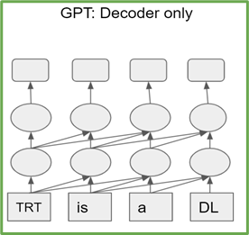
Transformer-based models are a stack of either transformer encoder or decoder blocks. Encoder (decoder) blocks have the same architecture and number of parameters. T5 consists of stacks of transformer encoders and decoders, while GPT-2 is composed of only transformer decoder blocks (Figure 1).
Figure 1a. T5 architecture
Figure 1b. GPT-2 architecture
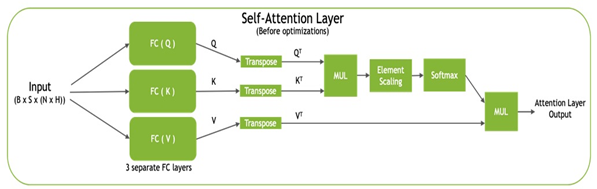
Each transformer block, also known as the self-attention block, consists of three projections by using fully connected layers to project the input into three different subspaces, termed query (Q), key (K), and value (V). These matrices are then transposed, with QT and KT being used to compute the normalized dot-product attention values, before being combined with VT to produce the final output (Figure 2).
Figure 2. Self-attention block
TensorRT optimizes the self-attention block by pointwise layer fusion:
Reduction is fused with power ops (for LayerNorm and residual-add layer).
Scale is fused with softmax.
GEMM is fused with ReLU/GELU activations.
Additionally, TensorRT also optimizes the network for inference:
Eliminating transpose ops.
Fusing the three KQV projections into a single GEMM.
When FP16 mode is specified, controlling layer-wise precisions to preserve accuracy while running the most compute-intensive ops in FP16.
TensorRT vs. PyTorch CPU and GPU benchmarks
With the optimizations carried out by TensorRT, we’re seeing up to 3–6x speedup over PyTorch GPU inference and up to 9–21x speedup over PyTorch CPU inference.
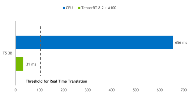
Figure 3 shows the inference results for the T5-3B model at batch size 1 for translating a short phrase from English to German. The TensorRT engine on an A100 GPU provides a 21x reduction in latency compared to PyTorch running on a dual-socket Intel Platinum 8380 CPU.
Figure 3. T5-3B model inference comparison. TensorRT on A100 GPU provides a 21x smaller latency compared to PyTorch CPU inference.
CPU: Intel Platinum 8380, 2 sockets. GPU: NVIDIA A100 PCI Express 80GB. Software: PyTorch 1.9, TensorRT 8.2.0 EA. Task: “Translate English to German: that is good.”
Conclusion
In this post, we walked you through converting the Hugging Face PyTorch T5 and GPT-2 models to an optimized TensorRT engine for inference. The TensorRT inference engine is used as a drop-in replacement for the original HuggingFace T5 and GPT-2 PyTorch models and provides up to 21x CPU inference speedup. To achieve this speedup for your model, get started today with TensorRT 8.2.
Torch-TensorRT is a PyTorch integration for TensorRT inference optimizations on NVIDIA GPUs. With just one line of code, it speeds up performance up to 6x on NVIDIA GPUs.
I’m excited about Torch-TensorRT, the new integration of PyTorch with NVIDIA TensorRT, which accelerates the inference with one line of code. PyTorch is a leading deep learning framework today, with millions of users worldwide. TensorRT is an SDK for high-performance, deep learning inference across GPU-accelerated platforms running in data center, embedded, and automotive devices. This integration enables PyTorch users with extremely high inference performance through a simplified workflow when using TensorRT.
Figure 1. PyTorch models can be compiled with Torch-TensorRT on various NVIDIA platforms
What is Torch-TensorRT
Torch-TensorRT is an integration for PyTorch that leverages inference optimizations of TensorRT on NVIDIA GPUs. With just one line of code, it provides a simple API that gives up to 6x performance speedup on NVIDIA GPUs.
This integration takes advantage of TensorRT optimizations, such as FP16 and INT8 reduced precision, while offering a fallback to native PyTorch when TensorRT does not support the model subgraphs.
How Torch-TensorRT works
Torch-TensorRT acts as an extension to TorchScript. It optimizes and executes compatible subgraphs, letting PyTorch execute the remaining graph. PyTorch’s comprehensive and flexible feature sets are used with Torch-TensorRT that parse the model and applies optimizations to the TensorRT-compatible portions of the graph.
After compilation, using the optimized graph is like running a TorchScript module and the user gets the better performance of TensorRT. The Torch-TensorRT compiler’s architecture consists of three phases for compatible subgraphs:
Lowering the TorchScript module
Conversion
Execution
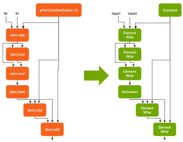
Lowering the TorchScript module
In the first phase, Torch-TensorRT lowers the TorchScript module, simplifying implementations of common operations to representations that map more directly to TensorRT. It is important to note that this lowering pass does not affect the functionality of the graph itself.
Figure 2. Parsing and transforming TorchScript’s graph
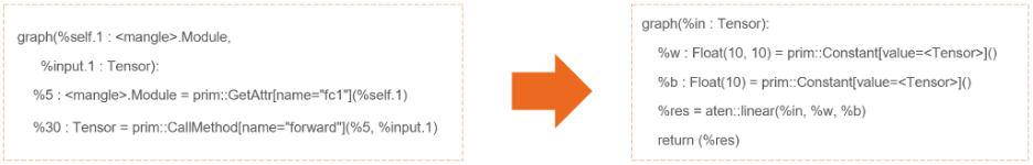
Conversion
In the conversion phase, Torch-TensorRT automatically identifies TensorRT-compatible subgraphs and translates them to TensorRT operations:
Nodes with static values are evaluated and mapped to constants.
Nodes that describe tensor computations are converted to one or more TensorRT layers.
The remaining nodes stay in TorchScripting, forming a hybrid graph that is returned as a standard TorchScript module.
Figure 3. Mapping Torch’s ops to TensorRT ops for the fully connected layer
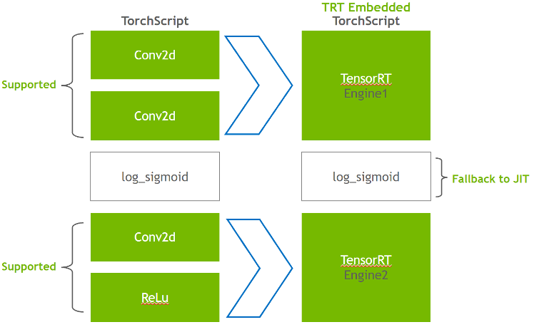
The modified module is returned to you with the TensorRT engine embedded, which means that the whole model—PyTorch code, model weights, and TensorRT engines—is portable in a single package.
Figure 4. Transforming the Conv2d layer into TensorRT engine while log_sigmoid falls back to TorchScript JIT
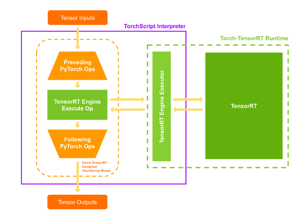
Execution
When you execute your compiled module, Torch-TensorRT sets up the engine live and ready for execution. When you execute this modified TorchScript module, the TorchScript interpreter calls the TensorRT engine and passes all the inputs. The engine runs and pushes the results back to the interpreter as if it was a normal TorchScript module.
Figure 5. Runtime execution of PyTorch and TensorRT ops
Torch-TensorRT features
Torch-TensorRT introduces the following features: support for INT8 and sparsity.
Support for INT8
Torch-TensorRT extends the support for lower precision inference through two techniques:
Post-training quantization (PTQ)
Quantization-aware training (QAT)
For PTQ, TensorRT uses a calibration step that executes the model with sample data from the target domain. IT tracks the activations in FP32 to calibrate a mapping to INT8 that minimizes the information loss between FP32 and INT8 inference. TensorRT applications require you to write a calibrator class that provides sample data to the TensorRT calibrator.
Torch-TensorRT uses existing infrastructure in PyTorch to make implementing calibrators easier. LibTorch provides a DataLoader and Dataset API, which streamlines preprocessing and batching input data. These APIs are exposed through C++ and Python interfaces, making it easier for you to use PTQ. For more information, see Post Training Quantization (PTQ).
For QAT, TensorRT introduced new APIs: QuantizeLayer and DequantizeLayer, which map the quantization-related ops in PyTorch to TensorRT. Operations like aten::fake_quantize_per_*_affine is converted into QuantizeLayer + DequantizeLayer by Torch-TensorRT internally. For more information about optimizing models trained with PyTorch’s QAT technique using Torch-TensorRT, see Deploying Quantization Aware Trained models in INT8 using Torch-TensorRT.
Sparsity
The NVIDIA Ampere architecture introduces third-generation Tensor Cores at NVIDIA A100 GPUs that use the fine-grained sparsity in network weights. They offer maximum throughput of dense math without sacrificing the accuracy of the matrix multiply accumulate jobs at the heart of deep learning.
TensorRT supports registering and executing some sparse layers of deep learning models on these Tensor Cores.
Torch-TensorRT extends this support for convolution and fully connected layers.
Example: Throughput comparison for image classification
In this post, you perform inference through an image classification model called EfficientNet and calculate the throughputs when the model is exported and optimized by PyTorch, TorchScript JIT, and Torch-TensorRT. For more information, see the end-to-end example notebook on the Torch-TensorRT GitHub repository.
Installation and prerequisites
To follow these steps, you need the following resources:
A Linux machine with an NVIDIA GPU, compute architecture 7 or earlier
Docker installed, 19.03 or earlier
A Docker container with PyTorch, Torch-TensorRT, and all dependencies pulled from the NGC Catalog
Now that you have a live bash terminal in the Docker container, launch an instance of JupyterLab to run the Python code. Launch JupyterLab on port 8888 and set the token to TensorRT. Keep the IP address of your system handy to access JupyterLab’s graphical user interface on the browser.
Navigate to this IP address on your browser with port 8888. If you are running this example of a local system, then navigate to Localhost:8888.
After you connect to JupyterLab’s graphical user interface on the browser, you can create a new Jupyter notebook. Start by installing timm, a PyTorch library containing pretrained computer vision models, weights, and scripts. Pull the EfficientNet-b0 model from this library.
pip install timm
Import the relevant libraries and create a PyTorch nn.Module object for EfficientNet-b0.
import torch
import torch_tensorrt
import timm
import time
import numpy as np
import torch.backends.cudnn as cudnn

torch.hub._validate_not_a_forked_repo=lambda a,b,c: True

efficientnet_b0 = timm.create_model('efficientnet_b0',pretrained=True)
You get predictions from this model by passing a tensor of random floating numbers to the forward method of this efficientnet_b0 object.
model = efficientnet_b0.eval().to("cuda")
detections_batch = model(torch.randn(128, 3, 224, 224).to("cuda"))
detections_batch.shape
This returns a tensor of [128, 1000] corresponding to 128 samples and 1,000 classes.
To benchmark this model through both PyTorch JIT and Torch-TensorRT AOT compilation methods, write a simple benchmark utility function:
cudnn.benchmark = True

def benchmark(model, input_shape=(1024, 3, 512, 512), dtype='fp32', nwarmup=50, nruns=1000):
    input_data = torch.randn(input_shape)
    input_data = input_data.to("cuda")
    if dtype=='fp16':
        input_data = input_data.half()

    print("Warm up ...")
    with torch.no_grad():
        for _ in range(nwarmup):
            features = model(input_data)
    torch.cuda.synchronize()
    print("Start timing ...")
    timings = []
    with torch.no_grad():
        for i in range(1, nruns+1):
            start_time = time.time()
            pred_loc  = model(input_data)
            torch.cuda.synchronize()
            end_time = time.time()
            timings.append(end_time - start_time)
            if i%10==0:
                print('Iteration %d/%d, avg batch time %.2f ms'%(i, nruns, np.mean(timings)*1000))

    print("Input shape:", input_data.size())
    print('Average throughput: %.2f images/second'%(input_shape[0]/np.mean(timings)))
You are now ready to perform inference on this model.
Inference using PyTorch and TorchScript
First, take the PyTorch model as it is and calculate the average throughput for a batch size of 1:
model = efficientnet_b0.eval().to("cuda")
benchmark(model, input_shape=(1, 3, 224, 224), nruns=100)
The same step can be repeated with the TorchScript JIT module:
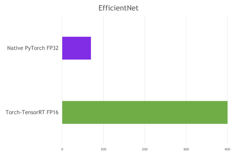
Here are the results that I’ve achieved on an NVIDIA A100 GPU with a batch size of 1.
Figure 6. Comparing throughput of native PyTorch with Torch-TensorRt on an NVIDIA A100 GPU with batch size 1
Summary
With just one line of code for optimization, Torch-TensorRT accelerates the model performance up to 6x. It ensures the highest performance with NVIDIA GPUs while maintaining the ease and flexibility of PyTorch.
Interested in trying it on your model? Download Torch-TensorRT from the PyTorch NGC container to accelerate PyTorch inference with TensorRT optimizations, and no code changes.
Learn about TensorRT 8.2 and the new TensorRT framework integrations, which accelerate inference in PyTorch and TensorFlow with just one line of code.
Today NVIDIA released TensorRT 8.2, with optimizations for billion parameter NLU models. These include T5 and GPT-2, used for translation and text generation, making it possible to run NLU apps in real time.
TensorRT is a high-performance deep learning inference optimizer and runtime that delivers low latency, high-throughput inference for AI applications. TensorRT is used across several industries including healthcare, automotive, manufacturing, internet/telecom services, financial services, and energy.
PyTorch and TensorFlow are the most popular deep learning frameworks having millions of users. The new TensorRT framework integrations now provide a simple API in PyTorch and TensorFlow with powerful FP16 and INT8 optimizations to accelerate inference by up to 6x.
Highlights include
TensorRT 8.2: Optimizations for T5 and GPT-2 run real-time translation and summarization with 21x faster performance compared to CPUs.
TensorRT 8.2: Simple Python API for developers using Windows.
Torch-TensorRT: Integration for PyTorch delivers up to 6x performance vs in-framework inference on GPUs with just one line of code.
TensorFlow-TensorRT: Integration of TensorFlow with TensorRT delivers up to 6x faster performance compared to in-framework inference on GPUs with one line of code.
Resources
Torch-TensorRT is available today in the PyTorch Container from the NGC catalog.
TensorFlow-TensorRT is available today in the TensorFlow Container from the NGC catalog.
Build an action recognition app with pretrained models, the TAO Toolkit, and DeepStream without large training data sets or deep AI expertise.
As humans, we are constantly on the move and performing several actions such as walking, running, and sitting every single day. These actions are a natural extension of our daily lives. Building applications that capture these specific actions can be extremely valuable in the field of sports for analytics, in healthcare for patient safety, in retail for a better shopping experience, and more.
However, building and deploying AI applications that can understand the temporal information of human action is challenging and time-consuming, requiring large amounts of training and deep AI expertise.
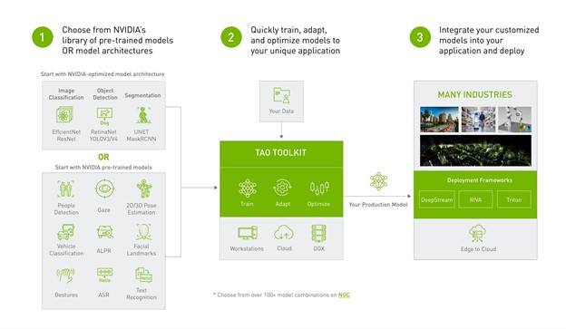
In this post, we show how you can fast-track your AI application development by taking a pretrained action recognition model, fine-tuning it with custom data and classes with the NVIDIA TAO Toolkit and deploying it for inference through NVIDIA DeepStream with no AI expertise whatsoever.
Figure 1. End-to-end workflow starting with a pretrained model, fine-tuning with the TAO Toolkit, and deploying it with DeepStream
Action recognition model
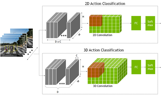
To recognize an action, the network must look at not just a single static frame but several consecutive frames. This provides the temporal context to understand the action. This is the extra temporal dimension compared to a classification or object detection model, where the network only looks at a single static frame.
These models are created using a 2D convolution neural network, where the dimensions are width, height, and number of channels. The 2D action recognition model is like the other 2D computer vision model, but the channel dimension now also contains the temporal information.
In the 2D action recognition model, you multiply the temporal frames D with the channel count C to form the channel dimension input.
For the 3D model, a new dimension, D, is added that represents the temporal information.
The output from both the 2D and 3D convolution networks goes into a fully connected layer, followed by a Softmax layer to predict the action.
Figure 2. Action recognition 2D and 3D convolution network
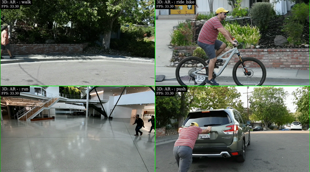
A pretrained model is one that has been trained on representative datasets and fine-tuned with weights and biases. The action recognition model, available from the NGC catalog, has been trained on five common classes:
Walking
Running
Pushing
Riding a bike
Falling
This is a sample model. More importantly, this model can then be easily retrained with custom data in a fraction of the time and data that it takes to train from scratch.
The pretrained model was trained on a few hundred short video clips from the HMDB51 dataset. For the five classes that the model is trained on, the 2D model achieved accuracy of 83% and the 3D model achieved an accuracy of 86%. Furthermore, the following table shows the expected performance on various GPUs, if you choose to deploy the model as-is.
Inference Performance (FPS)
2DResNet18
3DResNet18
Nano
30
0.6
NVIDIA Xavier NX
250
5
NVIDIA AGX Xavier
490
33
NVIDIA A30
5,809
356
NVIDIA A100
10,457
640
Table 1. Expected inference performance by model
For this experiment, you fine-tune the model with three new classes that consist of simple actions such as pushups, sit-ups, and pull-ups. You use the subset of HMDB51 dataset, which contains 51 different actions.
Prerequisites
Before you start, you must have the following resources for training and deploying:
In this section, you use the TAO Toolkit to fine-tune the model with the new classes.
The TAO Toolkit uses transfer learning, where it uses the learned features from an existing neural network model and applies it to a new one. A CLI and Jupyter notebook–based solution of the NVIDIA TAO framework, the TAO Toolkit abstracts away the AI/DL framework complexity, enabling you to create custom and production-ready models for your use case without any AI expertise.
You can either provide simple directives in the CLI window or use the turnkey Jupyter notebook for training and fine-tuning. You use the action recognition notebook from NGC to train your custom three-class model.
Download the version 1.3 of the TAO Toolkit Computer Vision Sample Workflows and unzip the package. In the /action_recognition_net directory, find the Jupyter notebook (actionrecognitionnet.ipynb) for action recognition training, and the /specs directory, which contains all the spec files for training, evaluation, and model export. You configure these spec files for training.
Start the Jupyter notebook and open the action_recognition_net/actionrecognitionnet.ipynb file:
All the training steps are run inside the Jupyter notebook. After you have started the notebook, run the Set up env variables and map drives and Install TAO launcher steps provided in the notebook.
Step 2: Download the dataset and pretrained model
After you have installed TAO, the next step is to download and prepare the dataset for training. The Jupyter notebook provides the steps to download and preprocess the HMDB51 dataset. If you have your own custom dataset, you can use it in step 2.1.
For this post, you use three classes from the HMDB51 dataset. Modify a few lines to add the push-up, pull-up, and sit-up classes.
$ wget -P $HOST_DATA_DIR http://serre-lab.clps.brown.edu/wp-content/uploads/2013/10/hmdb51_org.rar
$ mkdir -p $HOST_DATA_DIR/videos && unrar x $HOST_DATA_DIR/hmdb51_org.rar $HOST_DATA_DIR/videos
$ mkdir -p $HOST_DATA_DIR/raw_data
$ unrar x $HOST_DATA_DIR/videos/pushup.rar $HOST_DATA_DIR/raw_data
$ unrar x $HOST_DATA_DIR/videos/pullup.rar $HOST_DATA_DIR/raw_data
$ unrar x $HOST_DATA_DIR/videos/situp.rar $HOST_DATA_DIR/raw_data
The video files for each class are stored in their respective directory under $HOST_DATA_DIR/raw_data. These are encoded video files and must be uncompressed to frames to train the model. A script has been provided to help you prepare the data for training.
Download the helper scripts and install the dependency:
$ cd tao_recipes/tao_action_recognition/data_generation/
$ ./preprocess_HMDB_RGB.sh $HOST_DATA_DIR/raw_data  $HOST_DATA_DIR/processed_data
The output for each class is shown in the following code example. f cnt: 82 means that this video clip was uncompressed to 82 frames. This action is performed for all the videos in the directory. Depending on the number of classes and size of the dataset and video clips, this process can take some time.
Preprocess pullup
f cnt: 82.0
f cnt: 82.0
f cnt: 82.0
f cnt: 71.0
...
The format of the processed data looks something like the following code example. If you are training on your own data, make sure that your dataset also follows this directory format.
$HOST_DATA_DIR/processed_data/
|-->
|-->
The next step is to split the data into a training and validation set. The HMDB51 dataset provides a split file for each class, so just download that and divide the dataset into 70% training and 30% validation.
Use the helper script split_dataset.py to split the data. This only works with the split file provided with the HMDB dataset. If you are using your own dataset, then this wouldn’t apply.
$ cd tao_recipes/tao_action_recognition/data_generation/

$ python3 ./split_dataset.py $HOST_DATA_DIR/processed_data       $HOST_DATA_DIR/splits/testTrainMulti_7030_splits $HOST_DATA_DIR/train  $HOST_DATA_DIR/test
Data used for training is under $HOST_DATA_DIR/train and data for test and validation is under $HOST_DATA_DIR/test.
After preparing the dataset, download the pretrained model from NGC. Follow the steps in 2.1 of the Jupyter notebook.
$ ngc registry model download-version "nvidia/tao/actionrecognitionnet:trainable_v1.0" --dest $HOST_RESULTS_DIR/pretrained
Step 3: Configure training parameters
The training parameters are provided in the spec YAML file. In the /specs directory, find all the spec files for training, fine-tuning, evaluation, inference, and export. For training, you use train_rgb_3d_finetune.yaml.
For this experiment, we show you a few hyperparameters that you can modify. For more information about all the different parameters, see ActionRecognitionNet.
You can also overwrite any of the parameters during runtime. Most of the parameters are kept as default. The few that you are changing are highlighted in the following code block.
## Model Configuration
model_config:
   model_type: rgb
   input_type: "3d"
   backbone: resnet18
   rgb_seq_length: 32  ## Change from 3 to 32 frame sequence
   rgb_pretrained_num_classes: 5
   sample_strategy: consecutive
   sample_rate: 1

# Training Hyperparameter configuration
train_config:
   optim:
      lr: 0.001
      momentum: 0.9
      weight_decay: 0.0001
      lr_scheduler: MultiStep
      lr_steps: [5, 15, 25]
      lr_decay: 0.1
   epochs: 20  ## Number of Epochs to train
   checkpoint_interval: 1  ## Saves model checkpoint interval

## Dataset configuration
dataset_config:
   train_dataset_dir: /data/train  ## Modify to use your train dataset
   val_dataset_dir: /data/test     ## Modify to use your test dataset
   ## Label maps for new classes. Modify this for your custom classes
   label_map:
      pushup: 0
      pullup: 1
      situp: 2
For training, follow step 4 in the Jupyter notebook. Set your environment variables.
The TAO Toolkit task to train action recognition is called action_recognition. To train, use the tao action_recognition train command. Specify the training spec file and provide the output directory and pretrained model. Alternatively, you can also set the pretrained model in the model_config specs.
Depending on your GPU, sequence length or epochs, this can take anywhere from minutes to hours. Because you are saving every epoch, you see as many model checkpoints as the number of epochs.
The model checkpoints are saved as ar_model_epoch=-val_loss=.tlt. Pick the last epoch for model evaluation and export but you can use any that has the lowest validation loss.
Step 5: Evaluate the trained model
There are two different sampling strategies to evaluate the trained model on video clips:
Center mode: Picks up the middle frames of a sequence to do inference. For example, if the model requires 32 frames as input and a video clip has 128 frames, then you choose the frames from index 48 to index 79 to do the inference.
Conv mode: Convolutionally sample 10 sequences out of a single video and do inference. The results are averaged.
For evaluation, use the evaluation spec file (evaluate_rgb.yaml) provided in the /specs directory. This is like the training config. Modify the dataset_config parameter to use the three classes that you are training for.
dataset_config:
   ## Label maps for new classes. Modify this for your custom classes
   label_map:
      pushup: 0
      pullup: 1
      situp: 2
Evaluate using the tao action_recognition evaluate command. For video_eval_mode, you can choose between center mode or conv mode, as explained earlier. Use the last saved model checkpoint from the training run.
This was evaluated on a 90-video dataset, which had clips of all three actions. The overall accuracy is about 82%, which is decent for the size of the dataset. The larger the dataset, the better the model can generalize. You can try to test with your own clips for accuracy.
Step 6: Export for DeepStream deployment
The last step is exporting the model for deployment. To export, run the tao action_recognition export command. You must provide the export specs file, which is included in the /specs directory as export_rgb.yaml. Modify the dataset_config value in the export_rgb.yaml to use the three classes that you trained for. This is like dataset_config in evaluate_rgb.yaml.
$ tao action_recognition export
-e $SPECS_DIR/export_rgb.yaml
-k $KEY
model=$RESULTS_DIR/rgb_3d_ptm/ar_model_epoch=-val_loss=.tlt
/export/rgb_resnet18_3.etlt
Congratulations, you have successfully trained a custom 3D action recognition model. Now, deploy this model using DeepStream.
Deploying with DeepStream
In this section, we show how you can deploy the fine-tuned model using NVIDIA DeepStream.
The DeepStream SDK helps you quickly build efficient, high-performance video AI applications. DeepStream applications can run on edge devices powered by NVIDIA Jetson, on-premises servers, or in the cloud.
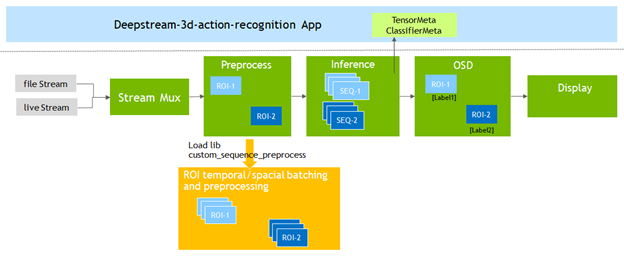
To support action recognition models, DeepStream 6.0 adds the Gst-nvdspreprocess plug-in. This plug-in loads a custom library (custom_sequence_preprocess.so) to perform temporal sequence catching and region of interest (ROI) partial batching and then forward the batched tensor buffers to the downstream inference plug-in.
You modify the deepstream-3d-action-recognition application included in the DeepStream SDK to test the model that you fine-tuned with TAO.
Figure 4. 3D action recognition application pipeline
The sample application runs inference on four video files simultaneously and presents the results with a 2×2 tiled display.
Run the standard application first before you do your modifications. First, start the DeepStream 6.0 development container:
For more information about the DeepStream containers available from NVIDIA, see the NGC catalog.
From within the container, navigate to the 3D action recognition application directory and download and install the standard 3D and 2D models from NGC.
Before modifying the application, familiarize yourself with the key configuration parameters of the preprocessor plug-in required to run the application.
From the /app/sample_apps/deepstream-3d-action-recognition folder, open the config_preprocess_3d_custom.txt file and review the preprocessor configuration for the 3D model.
Line 13 defines the 5-dimension input shape required by the 3D model:
network-input-shape = 4;3;32;224;224
For this application, you are using four inputs each with one ROI:
Your batch number is 4 (# of inputs * # of ROIs per input).
Your input is RGB so the number of channels is 3.
The sequence length is 32 and the input resolution is 224×224 (HxW).
Line 18 tells the preprocessor library that you are using a CUSTOM sequence:
network-input-order = 2
Lines 51 and 52 define how the frames are passed to the inference engine:
stride=1
subsample=0
A subsample value of 0 means that you pass on the frames sequentially (Frame 1, Frame 2, …) to the inference step.
A stride value of 1 means that there is a difference of a single frame between the sequences. For example:
Sequence A: Frame 1, 2, 3, 4, …
Sequence B: Frame 2, 3, 4, 5, …
Finally, lines 55 – 60 define the number of inputs and ROIs:
For more information about all the application and preprocessor parameters, see the Action Recognition section of the DeepStream documentation.
Running the new model
You are now ready to modify your application configuration and test the exercise action recognition model.
Because you’re using a Docker image, the best way to transfer files between the host filesystem and the container is to use the -v mount flag when starting the container to set up a shareable location. For example, use -v /home:/home to mount the host’s /home directory to the /home directory of the container.
Copy the new model, label file, and text video into the /app/sample_apps/deepstream-3d-action-recognition folder.
# back up the original labels file
$ cp ./labels.txt ./labels_bk.txt
$ cp /home/labels.txt ./
$ cp /home/Exercise_demo.mp4 ./
$ cp /home/rgb_resnet18_3d_exercises.etlt ./
Open deepstream_action_recognition_config.txt and change line 30 to point to the exercise test video.
Open config_infer_primary_3d_action.txt and change the model used for inference on line 63 and the batch size on line 68 from 4 to 1 because you are going from four inputs to a single input:
Finally, open config_preprocess_3d_custom.txt. Change the network-input-shape value to reflect the single input and configuration of the exercise recognition model on line 35:
network-input-shape= 1;3;3;224;224
Modify the source settings on lines 77 – 82 for a single input and ROI:
The action recognition sample application gives you the flexibility to change the input source, number of inputs, and model used without having to modify the application source code.
To review how the application was implemented, see the source code for the application, as well as the custom sequence library used by the preprocessor plug-in, in the /sources/apps/sample_apps/deepstream-3d-action-recognition folder.
Summary
In this post, we showed you an end-to-end workflow of fine-tuning and deploying an action recognition model using the TAO Toolkit and DeepStream, respectively. Both the TAO Toolkit and DeepStream are solutions that abstract away the AI framework complexity, enabling you to build and deploy AI applications in production without the need for any AI expertise.
Get started with your action recognition model by downloading the model from the NGC catalog.
For more information, see the following resources:
Movies like The Matrix and The Lord of the Rings inspired a lifelong journey in computer graphics for Piotr Skiejka, a senior visual effects artist at Ubisoft. Born in Poland and based in Singapore, Skiejka turned his childhood passion of playing with motion design — as well as compositing, lighting and rendering effects — into Read article >


 Explore NVIDIA Metropolis partners showcasing new technologies to improve city mobility at the ITS America 2021.
 Learn about the latest updates to NVIDIA TAO, an AI-model-adaptation framework, and NVIDIA TAO toolkit, a CLI and Jupyter notebook-based version of TAO.


 TensorRT 8.2 optimizes HuggingFace T5 and GPT-2 models. With TensorRT-accelerated GPT-2 and T5, you can generate excellent human-like texts and build real-time translation, summarization, and other online NLP applications within strict latency requirements.
 Torch-TensorRT is a PyTorch integration for TensorRT inference optimizations on NVIDIA GPUs. With just one line of code, it speeds up performance up to 6x on NVIDIA GPUs.
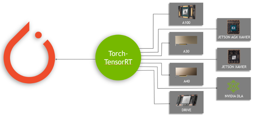
 Learn about TensorRT 8.2 and the new TensorRT framework integrations, which accelerate inference in PyTorch and TensorFlow with just one line of code.
 Build an action recognition app with pretrained models, the TAO Toolkit, and DeepStream without large training data sets or deep AI expertise.