
 In this post, we examine a method programmers can use to saturate memory bandwidth on a GPU.
Introduction
NVIDIA GPUs have enormous compute power and typically need to be fed data at high speed to deploy that power. That is possible, in principle, since GPUs also have high memory bandwidth, but sometimes they need the programmer’s help to saturate that bandwidth. In this blog post, we examine one method to accomplish that and apply it to an example taken from financial computing. We will explain under what circumstances this method can be expected to work well, and how to find out whether these circumstances apply to your workload.
Context
NVIDIA GPUs derive their power from massive parallelism. Many warps of 32 threads can be placed on a Streaming Multiprocessor (SM), awaiting their turn to execute. When one warp is stalled for whatever reason, the warp scheduler switches to another with zero overhead, making sure that the SM always has work to do. On the high-performance NVIDIA Ampere 100 (A100) GPU up to 64 active warps can share an SM, each with its own resources. On top of that, A100 has many SMs—108—that can all execute warp instructions simultaneously. Most instructions must operate on data, and that data almost always originates in the device memory (DRAM) attached to the GPU. One of the main reasons why even the abundance of warps on an SM can run out of work is because they are waiting on data to arrive from memory. If this happens and the bandwidth to memory is not fully utilized, it may be possible to reorganize the program to improve memory access and reduce warp stalls, which in turn makes the program complete faster.
First step: wide loads
In a previous blog post, we examined a workload that did not fully utilize the available compute and memory bandwidth resources of the GPU. We determined that prefetching data from memory before it is needed substantially reduced memory stalls and improved performance. When prefetching is not applicable, the quest is to determine what other factors may be limiting performance of the memory subsystem. One possibility is that the rate at which requests are made of that subsystem is too high. Intuitively, we may reduce the request rate by fetching multiple words per load instruction. It is best illustrated with an example.
In all code examples in this post, uppercase variables are compile-time constants. BLOCKDIMX assumes the value of the predefined variable blockDim.x. For some purposes, it must be a constant known at compile time, whereas for other purposes, it is useful for avoiding computations at run time.
The original code looked like this, where index is a helper function to compute array indices. It implicitly assumes that just a single, one-dimensional thread block is being used, which is not the case for the motivating application from which it was derived. However, it reduces code clutter and does not change the argument.
for (pt = threadIdx.x; pt Observe that each thread loads kmax consecutive values from the suggestively named small_array. This array is sufficiently small that it fits entirely in the L1 cache, but asking it to return data at a very high rate may become problematic. The following change recognizes that each thread can issue requests for two double-precision words in the same instruction if we restructure the code slightly and introduce the double2 data type, which is supported natively on NVIDIA GPUs; it stores two double-precision words in adjacent memory locations, which can be accessed with field selectors “x” and “y.” The reason this works is that each thread accesses successive elements of small_array. We call this technique wide loads. Notice that the inner loop over index “k” is now incremented by two instead of one.
for (pt = threadIdx.x; pt A few caveats are in order. First, we did not check whether kmax is even. If not, the modified loop over k would execute an extra iteration, and we would need to write some special code to prevent that. Second, we did not confirm that small_array is properly aligned on a 16-byte boundary. If not, the wide loads would fail. If it was allocated using cudaMalloc, it would automatically be aligned on a 256-byte boundary. But if it was passed to the kernel using pointer arithmetic, some checks would need to be carried out.
Next, we inspect the helper function index and discover that it is linear in pt with coefficient 1. Consequently, we can apply a similar wide-load approach to values fetched from big_array by requesting two double-precision values in one instruction. The difference between accesses to big_array and to small_array is that now successive threads within a warp access adjacent array elements. The restructured code below doubles the increment of the loop over elements of array big_array, and now each thread processes two array elements in each iteration.
for (pt = 2*threadIdx.x; pt The same caveats as before apply, and they should now be extended to parity of ptmax and alignment of big_array. Fortunately, the application from which this example was derived satisfies all the requirements. The figure below shows the duration (in nanoseconds) of a set of kernels that gets repeated identically multiple times in the application. The average speedup of the kernel was 1.63x for the combination of wide loads.

Second step: register use
We could be tempted to stop here and declare success, but a deeper analysis of the execution of the program, using NVIDIA Nsight Compute, shows that we have not fundamentally changed the rate of requests to the memory subsystem, even though we have halved the number of load instructions. The reason is that a warp load instruction—i.e. 32 threads simultaneously issuing load instructions—results in one or more sector requests, which is the actual unit of memory access processed by the hardware. Each sector is 32 bytes, so one warp load instruction of one 8-byte double-precision word per thread results in 8 sector requests (accesses are with unit stride), and one warp load instruction of double2 words results in 16 sector requests. The total number of sector requests is the same for plain and wide loads. So, what caused the performance improvement?
To understand the code behavior we need to consider a resource we have not yet discussed, namely registers. These are used to store the data loaded from memory and serve as input for arithmetic instructions. Registers are a finite resource. If a Streaming Multiprocessor (SM) hosts the maximum number of warps possible on the A100 GPU, 32 4-byte registers are available to each thread, which together can hold 16 double-precision words. The compiler that translates our code into machine language is aware of this and will limit the number of registers per thread. How do we determine the register use of our code and the role it plays in performance? We use the “source” view in Nsight Compute to see assembly code (“SASS”) and C source code side by side.
The innermost loop of the code is the one that is executed most, so if we select in the navigation menu “instructions executed” and subsequently ask to be taken to the line in the SASS code that has the highest number of those, we automatically land in the inner loop. If you are uncertain, you can compare SASS and the highlighted corresponding source code to confirm. Next, we identify in the SASS code of the inner loop all the instructions that load data from memory (LDG). Figure 2 shows a snippet of the SASS where we have panned around to find the start of the inner loop; it is on line 166 where the number of times an instruction is executed suddenly jumps to its maximum value.
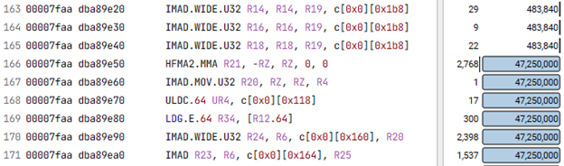
LDG.E.64 is the instruction we are after. It LoaDs from Global memory (DRAM) a 64-bit word with an Extended address. The load of a wide word corresponds to LDG.E.128. The first parameter after the name of the load instruction (R34 in Figure 2) is the register that receives the value. Since a double-precision value occupies two adjacent registers, R35 is implied in the load instruction. Next, we compare for the three versions of our code (1. baseline, 2. wide loads of small_array, 3. wide loads of small_array and big_array) the way registers are used in the inner loop. Recall that the compiler tries to stay within limits and sometimes needs to play musical chairs with the registers. That is, if not enough registers are available to receive each unique value from memory it will reuse a register previously used in the inner loop.
The effect of that is that the previous value needs to be used by an arithmetic instruction so that it can be overwritten by the new value. At this time the load from memory needs to wait until that instruction completes: a memory latency is exposed. On all modern computer architectures, this latency constitutes a significant delay. On the GPU some of it can be hidden by switching to another warp, but often not all of it. Consequently, the number of times a register is reused in the inner loop can be an indication of the slowdown of the code.
With this insight, we analyze the three versions of our code and find that they experience 8, 6, and 3 memory latencies per inner loop, respectively, which explains the differences in performance shown in Figure 1. The main reason behind the different register reuse patterns is that when two plain loads are fused into a single wide load, typically fewer address calculations are needed, and the result of an address calculation also goes into a register. With more registers holding addresses, fewer addresses are left over to act as “landing zones” for values fetched from memory, and we lose seats in the musical chairs game; the register pressure grows.
Third step: launch bounds
We are not yet done. Now that we know the critical role registers play in the performance of our program, we review total register use by the three versions of the code. Easiest is to inspect Nsight Compute reports again. We find that the numbers of registers used are 40, 36, and 44, respectively.
The way the compiler determines these numbers is by using sophisticated heuristics that take a large number of factors into account, including how many active warps may be present on an SM, the number of unique values to be loaded in busy loops, and the number of registers required for each operation. If the compiler has no knowledge of the number of warps that may be present on an SM, it will try to limit the number of registers per thread to 32, because that is the number that would be available if the absolute maximum simultaneous number of warps allowed by the hardware (64) were present. In our case we did not tell the compiler what to expect, so it did its best, but evidently determined that the code generated using just 32 registers would be too inefficient.
However, the actual size of the thread block specified in the launch statement of the kernel is 1024 threads, so 32 warps. This means that if only a single thread block is present on the SM, each thread can use up to 64 threads. At 40, 36, and 44 registers per thread of actual use, not enough registers would be available to support two or more thread blocks per SM, so exactly one will be launched, and we leave 24, 28, and 20 registers per thread unused, respectively.
We can do a lot better by informing the compiler of our intent through the use of launch bounds. By telling the compiler the maximum number of threads in a thread block (1024) and also the minimum number of blocks to support simultaneously (1), it relaxes and is happy to use 63, 56, and 64 registers per thread, respectively.
Interestingly, the fastest version of the code is now the baseline version without any wide loads. While the combined wide loads without launch bounds gave a speedup of 1.64x, with launch bounds the speedup with wide loads becomes 1.76x, whereas the baseline code speeds up by 1.77x. This means we did not have to go to the trouble of modifying the kernel definition; merely supplying launch bounds was enough in this case to obtain optimal performance for this particular thread block size.
Experimenting a little more with thread block sizes and minimum number of threads blocks to be expected on the SM, we reach a speedup of 1.79x at 2 thread blocks of 512 threads each per SM, also for the baseline version without wide loads.
Conclusions
Efficient use of registers is critical to obtaining good performance of GPU kernels. Sometimes a technique called “wide loads” can give significant benefits. It reduces the number of memory addresses that are computed and need to be stored in registers, leaving a larger number of registers to receive data from memory. However, giving the compiler hints about the way you launch kernels in your application may give the same benefit without having to change the kernel itself.
Acknowledgements
The author would like to thank Mark Gebhart and Jerry Zheng of NVIDIA for providing the expertise to analyze register use in the example discussed in this blog.