I load a really big image. I then downscale the image, and feed it to keras, who’s gonna perform filter = model.predict(image) on it. I then wanna take the results of model.predict(image) and be able to use it as a filter, i could apply to the original image
I want to do this since i have plenty of power for a 4k or even 6k image, but larger than that, and the model starts to struggle. But applying a 6k filter on a 8k, 10k or even 12k image doesn’t really affect the results at all (tested with good ol’ photoshop) So performing model.predict(image) on a lower res version, would save RAM, computational power, and a lot of time 🙂
Libraries and drivers are not one and the same. This blog explains which is the best for your need to clear up any confusion.
The NVIDIA DOCA Software framework includes everything needed to program the NVIDIA BlueField data processing unit (DPU) and provides a consistent experience regardless of the development environment. NVIDIA offers the following resources:
Developer Program
SDK manager support
A compilation of tools:
Compilers
Benchmarks
API reference and programmer’s guides
Reference applications
Use cases
NVIDIA delivers the stack by offering a DOCA SDK for developers and DOCA runtime software for out-of-the-box deployment.
DOCA drivers or DOCA libraries?
The DOCA drivers and DOCA libraries are critical pieces for developers, IT security and operations teams, and IT administrators. They are used to develop and deploy software-defined and hardware-accelerated applications for DPUs. However, I sometimes receive questions about the correct one to use.
To ensure that there is no confusion and to determine which might be best for your development needs, I’ve written this post to discuss when to use which.
DOCA drivers
DOCA libraries
Hardware-accelerated
Yes
Yes
Code management
Fine-grained control
Implicit initialization and unified APIs
Coding complexity
High complexity
Simplified, with programming guides
License
Mostly open source
DOCA
Multi-generation compatibility
Limited
Supported
Per-use case logic
Developers’ responsibility
Built-in
Reference applications
Partially available
Available for every library
Performance
Optimized
Maximized
Scale
Component dependent
Maximized
Table 1. DOCA drivers vs. DOCA libraries
Table 1 compares drivers and libraries and emphasizes the pros and cons of each. Essentially, DOCA drivers provide more room for customization, while DOCA libraries are architected to provide the best per-use case performance and scale with lower coding complexity.
DOCA libraries
First, DOCA libraries are higher-level abstraction APIs tuned for specific use cases. Libraries can be used to achieve outstanding performance with quicker development times and time-to-market. They also include a variety of guides and sample applications that provide a shorter learning curve than DOCA drivers when used for development.
NVIDIA libraries have been pre-accelerated. They enable you to build various applications quickly, with significant performance gains, as the logic has been created and tuned for designated use cases. They also ensure multi-generation compatibility, which can’t be guaranteed when using DOCA drivers.
The libraries aim to address a specific use case, such as a firewall, gateway, or storage controller. They use PMD and DPDK and contain additional functionality and logic that doesn’t exist within DPDK or at the driver level.
For example, if you use RegEx to identify complex string patterns for deep packet inspection (DPI), the DOCA DPI library includes preprocessing (packet header parsing) and post-processing routines to make it easier to use the RegEx accelerator to provide actions on network packets. The DPDK RegEx API does not include any of this. The DOCA DPI library API is abstracted and easier to develop packet inspection routines with, as there is no need to understand the logic.
DOCA libraries enable you to choose the preferred APIs with built-in hardware acceleration. The current revision of DOCA 1.3 includes over 120 DOCA APIs:
These services are available through the NGC Catalog and are deployable on BlueField DPUs in minutes.
The libraries’ value is delivered through a runtime environment, DOCA services, and an expansive set of documentation. The typical library user is not expected to develop applications but rather to leverage existing applications and services from NVIDIA or third parties.
DOCA services are containerized drivers and libraries made up of multiple items that can run as a service to provide specific functionality. Each service offers different capabilities, such as the DOCA telemetry API, which can be pulled in minutes from the NGC catalog. It provides a fast and convenient way to collect user-defined data and transfer it to DOCA telemetry service (DTS).
In addition, the API offers several built-in outputs for user convenience, including saving data directly to storage, NetFlow, Fluent Bit forwarding, and Prometheus endpoint.
Each of these libraries share objects and are not tied in any way except that they each use the PMD driver. Similarly, each has a common infrastructure, and each has its own documentation and programmer’s guide.
DOCA drivers and DOCA SDK
Although libraries eliminate low-level programming, they may not support all features and functionality that you are looking for, so NVIDIA offers DOCA drivers. DOCA drivers are open source-based and provide more flexibility if you’re developing yourown solutions or must create a unique solution.
NVIDIA drivers are designed for developers and are delivered through the DOCA SDK. The SDK includes all the components required to create and build applications, including reference application sources, development tools, documentation, and the NVIDIA SDK manager. The SDK manager enables the quick deployment of the development environment and can also flash and install an image to a local DPU.
The developer container enables the development of DOCA-accelerated applications anywhere. You don’t have to do this on the Arm processors on the DPU. On a host with the physical DPU, you can do this in a developer container, which emulates the Arm processor. NVIDIA provides detailed documentation, examples, and API compatibility.
The DOCA SDK is the most efficient way for you to leverage the DOCA libraries and drivers and create unique and personalized software to meet your application development needs.
The DOCA runtime is also available for you to verify and test your applications.
DOCA Runtime
If you’re unready or unable to port your application to the Arm architecture, NVIDIA provides the DOCA runtime for x86. In this case, a gRPC client runs on the DPU and establishes a communications channel with the x86 runtime. The application can access DPU runtime components, and you don’t have to compile any Arm code.
DOCA simplifies the programming and application development for BlueField DPUs and removes obstacles by providing a higher level of abstraction. By providing runtime binaries and high-level APIs, the DOCA framework enables you to focus on application code rather than learning.
There are two development routes you can choose: through libraries and services or through an SDK and drivers. Currently, the DOCA software stack includes over 120 DOCA APIs that are being used by more than 2500 DOCA developers worldwide. They are available through the NGC Catalog.
If you are new to DOCA, NVIDIA offers a complimentary, self-paced course, Introduction to DOCA for DPUs. It covers the essentials of the DOCA platform.
I hope I’ve cleared up any confusion and I encourage you to start your development journey by joining the DOCA developer program today.
For more information, see the following resources:
NVIDIA Holoscan for HPC brings AI to edge computing. Streaming Reactive Framework will be released in June to simplify code changes to stream AI for instrument processing workflows.
Scientific instruments are being upgraded to deliver 10–100x more sensitivity and resolution over the next decade, requiring a corresponding scale-up for storage and processing. The data produced from these enhanced instruments will reach limits that Moore’s law cannot adequately address and it will challenge traditional operating models solely based upon HPC in data centers.
Introducing the NVIDIA Holoscan platform for HPC Edge
The NVIDIA Holoscan platform has expanded to meet the specific needs of DevOps engineers, performance engineers, data scientists, and researchers working at these incredible edge instruments.
Modern real-time, edge AI applications are increasingly becoming multimodal. They involve high-speed IO, vision AI, imaging AI, graphics, streaming technologies, and more. Creating and maintaining these applications is extremely difficult. Scaling them is even harder.
NVIDIA is building the Streaming Reactive Framework (SRF) to address these challenges.
Figure 1. NVIDIA Holoscan for HPC workflow
While it was initially targeted at healthcare, Holoscan is a universal computation and imaging platform built for high performance while meeting the Size-Weight-and-Power (SWaP) constraints at the edge.
Now, the Holoscan platform has been extended, thanks to an easy-to-use software framework that maximizes developer productivity by ensuring maximum streaming data performance and computation. The platform is cloud-native and supports hybrid computing and data pipelining between edge locations and data centers. It is also architected for scalability, using network-aware optimizations and asynchronous computation.
The extended Holoscan platform delivers a flexible software stack that can run on embedded devices based on the NVIDIA Jetson AGX Xavier or Jetson AGX Orin. There is also a cloud-native version that runs on common high-performance hardware to accelerate data analysis and visualization workflows at the edge.
Introducing the NVIDIA Streaming Reactive Framework
The finest minds in HPC and AI research are continuously developing faster and better algorithms to solve today’s most challenging problems. However, many developers find it challenging to port their models and codes to full-rate production, particularly when faced with high-rate streaming input and strict throughput and latency requirements.
An effective solution requires a myriad of skill sets: talent coming from data scientists to performance engineers while spanning multiple software languages, hardware and software architectures, localities, and scaling rules. As a result, NVIDIA created the streaming reactive framework (SRF) to ease the research-to-production burden while maintaining speed-of-light performance.
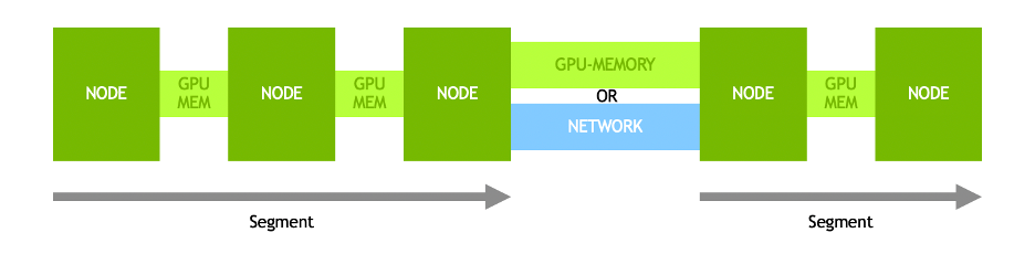
Figure 2. Within Holoscan, the HPC streaming data pipelines are standardized, using SRF, for building a modular and reusable pipeline for sensor data
NVIDIA SRF is a network-aware, flexible, and performance-oriented streaming data framework that standardizes and simplifies cloud-to-edge production HPC and AI deployments for C++ and Python developers alike.
When you build an NVIDIA SRF pipeline, specify the application data flow. along with scaling and placement logic. The placement logic dictates what hardware a data flow runs, and the scaling logic expresses how many parallel copies are needed to meet performance requirements.
NVIDIA SRF easily integrates with both C++ and Python code along with the NVIDIA catalog of domain-specific SDKs.
NVIDIA SRF is still in its experimental phase and is under active development. You can download NVIDIA SRF on GitHub in mid-June 2022.
AI for visualization and imaging
NVIDIA Orin, a low-power system-on-chip based on the NVIDIA Ampere architecture, set new records in AI inference, raising the bar in per-accelerator performance at the edge. It ran up to 5x faster than the previous generation Jetson AGX Xavier, while delivering an average of 2x better energy efficiency.
Jetson AGX Orin is a key ingredient in Holoscan for HPC and NVIDIA Clara Holoscan, a platform system makers and researchers are using to develop next-generation AI instruments. Its powerful computation capabilities for imaging and its versatile software stack makes it appealing to HPC edge use cases involving visualization and imaging.
With its JetPack SDK, Orin runs the full NVIDIA AI platform, a software stack already proven in the data center and the cloud. It is backed by a million developers using the NVIDIA Jetson platform.
The Advanced Photon Source (APS) at the US Department of Energy’s Argonne National Laboratory produces ultrabright, high-energy photon beams. The photons are 100 billion times brighter than a standard hospital X-ray machine and can capture images at the nano and atomic scale. With its APS-U upgrade in 2024, it will be able to generate photons that are up to 500x brighter than the current machine.
The Diamond Light Source at Oxford is a world-class synchrotron facility and is upgrading its brightness and coherence, up to 20 times, across existing beamlines plus five new flagship beamlines. Data rates from Diamond are already petabytes per month and, with Diamond-II, are expected to be at least an order of magnitude greater.
Worldwide, there are over 50 advanced light sources supporting the work of more than 16,000 researcher scientists and there are many more upgrades occurring at these instruments as well. While all these advancements are remarkable in their own accord, they are dependent on computational and data scientists to be ready with their AI-enabled data processing applications running on supercomputers at the edge.
PtychoNN: The APS edge computing platform
The APS is a machine about the size of a football field that produces photon beams. The beams are used to study materials, physics, and biological structures.
Today, one way of generating images of a material with nanoscale resolution is ptychography, a computationally intensive method to convert scattered X-ray interference patterns into images of the actual object.
To date, the method requires solving a challenging inverse problem, namely using forward and inverse Fourier transforms to iteratively compute the image of the object from the diffraction patterns observed in tens of thousands of X-ray measurements. Scientists wait for days just to get the experiment image results.
Now, with AI, scientists can bypass much of the inversion process and view images of the object while the experiment is running, even potentially making adjustments on-the-fly.
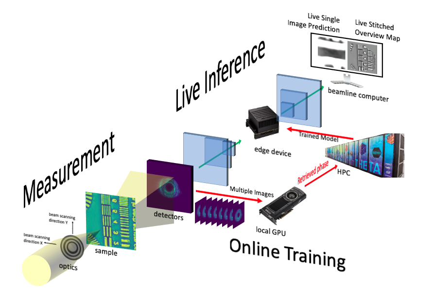
With AI, APS scientists were able to use a streaming ptychography pipeline, accelerated by a deep convolutional neural network model, PtychoNN, to speed up image processing by over 300x and reduce the data required to produce high-quality images by 25x.
Figure 3. Train the PtychoNN model at the data center on A100s and deploy the trained AI model at the beamline instrument with AGX Orin running PtychoNN to stream images 300x faster
The PtychoNN model is trained on NVIDIA A100 Tensor Core GPUs with deep learning and X-ray image phase-retrieval data. The trained model can run on an edge appliance to directly map the incoming diffraction images to images of the object in real space and in real time in only milliseconds.
Faster sampling means more productive use of the instrument, delivering opportunities to investigate more materials. It provides capabilities not possible before, such as looking at biological materials samples that were damaged in the X-ray beam, samples that are changing rapidly, or samples that are large compared to the size of the X-ray beam.
A common hardware and software architecture simplifies orchestration with NVIDIA AGX at the edge and clusters of A100 GPUs in the data center. The solution is easily extensible to keep up with the 125x increase in data rate expected at the APS. The increase is expected from a detector upgrade in 2022 and a facility upgrade in 2024.
“In order to make full use of what the upgraded APS will be capable of, we have to reinvent data analytics. Our current methods are not enough to keep up. Machine learning can make full use and go beyond what is currently possible.”
Mathew Cherukara, Argonne National Laboratory Computational Scientist
In the example earlier, a single GPU edge device accelerates a stream of images using a trained neural network. Turnaround times for edge experiments that took days can now take fractions of a second, providing researchers with real-time interactive use of their large-scale scientific instruments. For more information about other relevant HPC and AI at the edge examples, see the following resources:
While many of our highlighted edge HPC applications are focused on streaming video and imaging pipelines, NVIDIA Holoscan can be extended to other sensor types with a variety of data formats and rates. Whether you are performing high-bandwidth spectrum analysis with a software-defined radio or monitoring telemetry from a power grid for anomalies, NVIDIA Holoscan is the platform of choice for software-defined instruments.
By focusing on developer productivity and application performance regardless of the sensor, HPC at the edge can provide real-time analytics and mission success.
Featured image courtesy of US Department of Energy’s Argonne National Laboratory, Advanced Photon Source (APS)
Celebrate the onset of summer this GFN Thursday with 25 more games joining the GeForce NOW library, including seven additions this week. Because why would you ever go outside? Looking to spend the summer months in Space Marine armor? Games Workshop is kicking off its Warhammer Skulls event for its sixth year, with great discounts Read article >
Hello,I would like to know if tflite conversion includes any quantisation of the model parameters or is only a transformation of the format in which the model is stored?
Hello, I want to build a CNN with TensorFlow, I want to load the data with image_dataset_from_directory, and I have the labels, a list of numbers from 0 to 3, so I expect to TensorFlow tell me that it found N images and 4 classes, but I show me that it found 321 classes.
The labels list is like: [0, 3, 1, 1, … , 2, 0, 0]
So, I don’t know if I should modify the list format o distribution, or add another parameter in image_dataset_from_directory, if someone can help me please 🙁
So I started flowing the TensorFlow pip install guide however when it comes to actually checking if it can see the GPU it always comes back with this
(tf) C:UsersShain>python3 -c "import tensorflow as tf; print(tf.reduce_sum(tf.random.normal([1000, 1000])))" 2022-06-01 21:27:36.605396: W tensorflow/stream_executor/platform/default/dso_loader.cc:64] Could not load dynamic library 'cudart64_110.dll'; dlerror: cudart64_110.dll not found 2022-06-01 21:27:36.605523: I tensorflow/stream_executor/cuda/cudart_stub.cc:29] Ignore above cudart dlerror if you do not have a GPU set up on your machine. WARNING:tensorflow:Please fix your imports. Module tensorflow.python.training.tracking.base has been moved to tensorflow.python.trackable.base. The old module will be deleted in version 2.11. WARNING:tensorflow:Please fix your imports. Module tensorflow.python.training.checkpoint_management has been moved to tensorflow.python.checkpoint.checkpoint_management. The old module will be deleted in version 2.9. WARNING:tensorflow:Please fix your imports. Module tensorflow.python.training.tracking.resource has been moved to tensorflow.python.trackable.resource. The old module will be deleted in version 2.11. WARNING:tensorflow:Please fix your imports. Module tensorflow.python.training.tracking.util has been moved to tensorflow.python.checkpoint.checkpoint. The old module will be deleted in version 2.11. WARNING:tensorflow:Please fix your imports. Module tensorflow.python.training.tracking.base_delegate has been moved to tensorflow.python.trackable.base_delegate. The old module will be deleted in version 2.11. WARNING:tensorflow:Please fix your imports. Module tensorflow.python.training.tracking.graph_view has been moved to tensorflow.python.checkpoint.graph_view. The old module will be deleted in version 2.11. WARNING:tensorflow:Please fix your imports. Module tensorflow.python.training.tracking.python_state has been moved to tensorflow.python.trackable.python_state. The old module will be deleted in version 2.11. WARNING:tensorflow:Please fix your imports. Module tensorflow.python.training.saving.functional_saver has been moved to tensorflow.python.checkpoint.functional_saver. The old module will be deleted in version 2.11. WARNING:tensorflow:Please fix your imports. Module tensorflow.python.training.saving.checkpoint_options has been moved to tensorflow.python.checkpoint.checkpoint_options. The old module will be deleted in version 2.11. 2022-06-01 21:27:38.504483: W tensorflow/stream_executor/platform/default/dso_loader.cc:64] Could not load dynamic library 'cudart64_110.dll'; dlerror: cudart64_110.dll not found 2022-06-01 21:27:38.504803: W tensorflow/stream_executor/platform/default/dso_loader.cc:64] Could not load dynamic library 'cublas64_11.dll'; dlerror: cublas64_11.dll not found 2022-06-01 21:27:38.507542: W tensorflow/stream_executor/platform/default/dso_loader.cc:64] Could not load dynamic library 'cublasLt64_11.dll'; dlerror: cublasLt64_11.dll not found 2022-06-01 21:27:38.508572: W tensorflow/stream_executor/platform/default/dso_loader.cc:64] Could not load dynamic library 'cufft64_10.dll'; dlerror: cufft64_10.dll not found 2022-06-01 21:27:38.509170: W tensorflow/stream_executor/platform/default/dso_loader.cc:64] Could not load dynamic library 'curand64_10.dll'; dlerror: curand64_10.dll not found 2022-06-01 21:27:38.509519: W tensorflow/stream_executor/platform/default/dso_loader.cc:64] Could not load dynamic library 'cusolver64_11.dll'; dlerror: cusolver64_11.dll not found 2022-06-01 21:27:38.509902: W tensorflow/stream_executor/platform/default/dso_loader.cc:64] Could not load dynamic library 'cusparse64_11.dll'; dlerror: cusparse64_11.dll not found 2022-06-01 21:27:38.510368: W tensorflow/stream_executor/platform/default/dso_loader.cc:64] Could not load dynamic library 'cudnn64_8.dll'; dlerror: cudnn64_8.dll not found 2022-06-01 21:27:38.510665: W tensorflow/core/common_runtime/gpu/gpu_device.cc:1867] Cannot dlopen some GPU libraries. Please make sure the missing libraries mentioned above are installed properly if you would like to use GPU. Follow the guide at https://www.tensorflow.org/install/gpu for how to download and setup the required libraries for your platform. Skipping registering GPU devices... 2022-06-01 21:27:38.511499: I tensorflow/core/platform/cpu_feature_guard.cc:193] This TensorFlow binary is optimized with oneAPI Deep Neural Network Library (oneDNN) to use the following CPU instructions in performance-critical operations: AVX AVX2 To enable them in other operations, rebuild TensorFlow with the appropriate compiler flags. tf.Tensor(1560.4835, shape=(), dtype=float32)
I’ve tried setting an environment variable in the anaconda environment via
conda env config vars set EnvironmentBin=%CONDA_PREFIX%Librarybin
to see if it would help point tensor flow to the DLLs but that didn’t work either
not entirely sure what I am meant to do from here.
Using Numba and PyOptiX, NVIIDA enables you to configure ray tracing pipeline and write kernels in Python compatible with the OptiX pipeline.
Ray tracing is a rendering algorithm that can generate photorealistic images by simulating how light transmits and interacts with different materials. Today, it is widely adopted to bring imagery to life in game development, film-making, and physics simulations.
However, the ray-tracing algorithm is computationally intensive and requires hardware acceleration on the GPU to achieve real-time performance.
To leverage the hardware power for ray tracing, various toolchains and languages were invented to suit the need, such as openGL and the shading language.
Often, the build process of these software toolchains poses significant challenges to Python developers. To alleviate the difficulty and provide a familiar environment for writing ray tracing kernels, NVIDIA developed the Numba extension for PyOptiX. This extension enables graphics researchers and application developers to reduce the time from idea to implementation and shorten the development cycle on each iteration.
In this post, I provide an overview of the NVIDIA ray-tracing engine PyOptiX and explain how the Python JIT compiler, Numba, accelerates Python code. Finally, with a complete ray tracing example, I walk you through the steps of using the Numba extension for PyOptiX and write an accelerated ray tracing kernel in Python.
What are NVIDIA OptiX and PyOptiX?
NVIDIA RTX technology made ray tracing the default rendering algorithm in many modern rendering pipelines. As the demand for unique looks is unlimited, there’s a need for flexibility in customizing the rendering pipeline.
The NVIDIA RTX ray-tracing pipeline is customizable. By configuring how light transmits, reflects, and refracts on various materials, you can achieve distinctive looks on objects, such as shiny, glossy, or semi-transparent. By configuring how light rays are generated, you change the field of view and perspective of the look accordingly.
To address this need, NVIDIA developed NVIDIA OptiX, a ray-tracing engine that enables you to configure a hardware-accelerated ray-tracing pipeline. PyOptiX is the NVIDIA OptiX Python interface. This interface offers the capability for Python developers to have the same capabilities as NVIDIA OptiX developers who write in C++.
Kernel functions
To customize image facets, you use kernel functions, also referred to as kernel methods or kernels. You can think of kernels as a group of algorithms that transform data inputs to the required form. Native NVIDIA OptiX developers can write kernels with CUDA. With a Numba extension, you can write ray-tracing kernels in Python.
Higher performance with Numba and Numba.cuda
Ray tracing is a compute-intensive algorithm. While it is theoretically possible to run the ray-tracing kernel with the standard CPython interpreter, it would take days to render a regular ray-traced image. Moreover, NVIDIA OptiX requires the kernel to be runnable on a GPU device so that it integrates with the rest of the rendering pipeline.
Using Numba, a just-in-time Python function compiler, you can execute and accelerate your Python ray-tracing kernels with GPU hardware. Numba parses the Python function code and converts it to efficient machine code. On a high level, this process is divided into seven steps:
The function’s byte code is generated with the bytecode compiler.
The bytecode is analyzed. The control flow graph (CFG) and the data flow graph (DFG) are generated.
With bytecode, CFG, and DFG, the Numba intermediate representation (IR) is generated.
Based on the type of function inputs, the type is inferred for each IR variable.
The Numba IR is rewritten and gets Python-specific optimization.
The Numba IR is lowered to the LLVM IR, and more general optimization is performed.
The LLVM IR is consumed by the LLVM backend and optimized GPU machine code is generated.
Figure 1. A high-level view of Numba’s compilation pipeline
Because Numba can convert any Python functions into native code, in a Numba CUDA kernel, Python users have equal power as if they are writing the kernel in native CUDA. This code shows a dot product that’s executable on the device. For more information, see Numba Examples.
Introducing the Numba extension for PyOptiX
To customize specific stages of the ray-tracing pipeline, you must translate the Numba kernel into something that can be understood by the NVIDIA OptiX engine. NVIDIA developed the Numba Extension for PyOptiX to achieve this goal.
The extension includes custom type definition and intrinsic function lowerings. NVIDIA OptiX comes with a set of internal types:
OptixTraversableHandle
OptixVisibilityMask
SbtDataPointer
Functions such as optix.Trace
For Numba to perform type inference on these new types and methods, you must register these types and provide an implementation of these methods before compiling the user kernel. Currently, NVIDIA is expanding supported types and intrinsics to add more examples.
By exposing these types and intrinsics to Numba, you can now write kernels, which not only target the GPU but can specifically target the GPU for ray-tracing kernels. In combination with Numba CUDA, you can write ray-tracing kernels of equal power as if you were writing native CUDA ray-tracing kernels for NVIDIA OptiX.
In the next section, I introduce a Hello World example with the PyOptiX Numba extension. Before that, let me quickly go over some ray-tracing algorithm basics.
Fundamentals of ray tracing
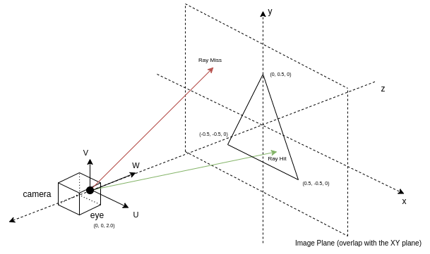
Imagine that you use a camera to capture an image. The light source in the scene emits light rays, which travel in a straight line. When a light ray hits an object, it is reflected from the surface and eventually reaches the camera sensor.
From a high level, a ray-tracing algorithm walks through all rays that reach the image plane to identify in the scene where and what the ray intersects with. When the intersection point is found, you can adopt various shading techniques to determine the color of the intersected point. However, there are also rays that don’t hit anything in the scene. In this case, these rays are considered as “missing” the target.
Steps for ray tracing a triangle with the Numba extension for PyOptiX
In the following example, I show how the Numba extension for PyOptiX can help you write custom kernels to define the ray behavior at ray generation, ray hit, and ray miss.
Scene setup
I modeled the view you see as an image plane, which usually sits slightly in front of the camera. The camera is modeled as a point and a set of mutually orthogonal vectors in the 3D space.
Figure 2. Scene setup for the triangle rendering example
Camera
The camera is modeled as a point in three dimensions. The three vectors, U, V, and W, are used to show the sideways, upwards, and frontal directions of the camera. This uniquely determines the position and orientation of the camera.
To simplify the computation for ray generation later, the U and V vectors are not unit vectors. Instead, their lengths proportionally match the image’s aspect ratio. Lastly, the length of the W vector is the distance between the camera and the image plane.
Ray generation kernel
The ray generation kernel is the centerpiece of the algorithm. Ray origins and directions are generated here and then passed down to the trace call. Its intensity is retrieved from other kernels and written as image data. In this section, I discuss the methods used to generate rays in this kernel.
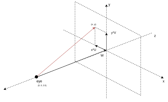
With the camera and the image plane, you can generate the rays. Adopt a coordinate system convention where the center of the image is the origin. The sign of a coordinate in an image pixel shows its relative position to the origin and its magnitude shows the distance. With this property, multiply the camera’s U and V vector with the corresponding elements of the pixel position and add them together. The result is a vector that points to the pixel from the image center.
Finally, add this vector to the W or front vector, and this generates a ray that originates at the camera position and goes through the pixel on the image plane. Figure 3 shows the decomposition of a ray that originates from the camera and goes through point (x, y) in the image plane.
Figure 3. Decomposition of a ray that goes through pixel (x, y)
In code, the pixel index and image dimension of the image plane can be retrieved using two optix intrinsic functions optix.GetLaunchIndex and optix.GetLaunchDimensions. Next, the pixel index is normalized to [-1.0, 1.0]. The following code example shows this logic in the Numba CUDA kernel.
@cuda.jit(device=True, fast_math=True)
defcomputeRay(idx, dim):
   U = params.cam_u
   V = params.cam_v
   W = params.cam_w
   # Normalizing coordinates to [-1.0, 1.0]
   d = float32(2.0) * make_float2(
       float32(idx.x) / float32(dim.x), float32(idx.y) / float32(dim.y)
   ) - float32(1.0)

   origin = params.cam_eye
   direction = normalize(d.x * U + d.y * V + W)
   return origin, direction

def __raygen__rg():
   # Look up your location within the launch grid
   idx = optix.GetLaunchIndex()
   dim = optix.GetLaunchDimensions()

   # Map your launch idx to a screen location and create a ray from the camera
   # location through the screen
   ray_origin, ray_direction = computeRay(make_uint3(idx.x, idx.y, 0), dim)
This code example shows the helper function of computeRay that computes the origin and direction vector of the ray.
Next, pass the generated ray into the intrinsic function optix.Trace. This initializes the ray tracing algorithm. The underlying optiX engine traverses through the primitives, computes the intersection point in the scene, and finally returns the intensity of the ray. The following code example shows the call to optix.Trace.
# In __raygen__rg
   payload_pack = optix.Trace(
       params.handle,
       ray_origin,
       ray_direction,
       float32(0.0),  # Min intersection distance
       float32(1e16), # Max intersection distance
       float32(0.0),  # rayTime -- used for motion blur
       OptixVisibilityMask(255), # Specify always visible
       uint32(OPTIX_RAY_FLAG_NONE),
       uint32(0),  # SBT offset   -- Refer to OptiX Manual for SBT
       uint32(1), # SBT stride   -- Refer to OptiX Manual for SBT
       uint32(0),  # missSBTIndex -- Refer to OptiX Manual for SBT
   )
Ray hit kernel
In the ray hit kernel, you write code to determine the intensity of each channel of the light ray. If the triangle vertices are set up using the NVIDIA OptiX internal data structure, then you can call the NVIDIA OptiX intrinsic optix.GetTriangleBarycentrics to retrieve the barycentric coordinates of the hit point.
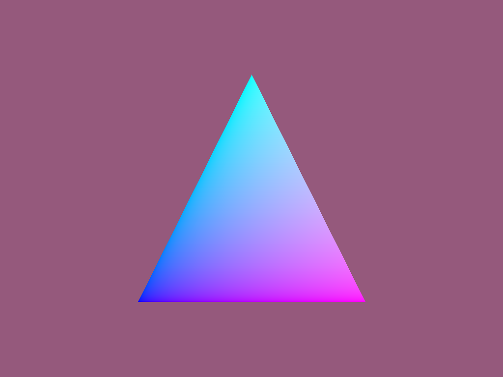
To make the color more interesting, insert this coordinate into the color for that pixel. The blue channel of the color is set to 1.0. The intensity of the ray should be passed to the ray generation kernel for further post-processing and be written to the image.
NVIDIA OptiX shares data between the kernels through payload registers. Use the setPayload function to set the values of the payload registers to the ray intensities. By default, payload registers are integer types. Use the CUDA intrinsic float_as_int to interpret the float value as an integer, without changing the bits.
@cuda.jit(device=True, fast_math=True)
defsetPayload(p):
   optix.SetPayload_0(float_as_int(p.x))
   optix.SetPayload_1(float_as_int(p.y))
   optix.SetPayload_2(float_as_int(p.z))

def__closesthit__ch():
   # When a built-in triangle intersection is used, a number of fundamental
   # attributes are provided by the NVIDIA OptiX API, including barycentric coordinates.
   barycentrics = optix.GetTriangleBarycentrics()

   setPayload(make_float3(barycentrics, float32(1.0)))
Ray miss kernel
The ray miss kernel sets the color of the rays that didn’t hit any objects in the scene. Here you set them to the background color.
bg_color is some data specified in the shader-binding table during the setup of the render pipeline. For now, just be aware that it’s a set of hard-coded floats representing the background color of the scene.
You have now defined the color for all rays. The color is retrieved in the ray generation kernel as a payload_pack data structure from the optix.trace call. Remember that in the ray hit and the ray miss kernel, you had to interpret the bits of the floating-point numbers into integers? Revert this step with the int_as_float function.
Now, you may directly write these values to the image and it would still look great. Take an extra step of performing post-processing steps to raw pixel values, which are important to great images in more complicated scenes.
The values that you have retrieved are simply raw intensities of the ray, which scale linearly to the energy level that the ray carries. While this fits your physical world’s model, the human eye does not respond to light stimuli in a linear fashion. Instead, it follows the mapping of input to respond by a power function.
To account for this, perform a gamma correction to the intensities. In addition, most users who are viewing the result of this image are watching a monitor with sRGB color space. Assume that the values from the ray-tracing world are in CIE-XYZ color space, and apply a color space conversion. Finally, perform quantization of the color values into 8-bit unsigned integers.
The following code example shows the helper functions for post-processing color intensities and writing them to the pixel array in the ray-generation kernel.
@cuda.jit(device=True, fast_math=True)
deftoSRGB(c):
   # Use float32 for constants
   invGamma = float32(1.0) / float32(2.4)
   powed= make_float3(
       fast_powf(c.x, invGamma),
       fast_powf(c.y, invGamma),
       fast_powf(c.z, invGamma),
   )
   return make_float3(
       float32(12.92) * c.x
       if c.x  float32(0.0031308)
       else float32(1.055) * powed.x - float32(0.055),
       float32(12.92) * c.y
       if c.y  float32(0.0031308)
       else float32(1.055) * powed.y - float32(0.055),
       float32(12.92) * c.z
       if c.z  float32(0.0031308)
       else float32(1.055) * powed.z - float32(0.055),
   )

@cuda.jit(device=True, fast_math=True)
defmake_color(c):
   srgb= toSRGB(clamp(c, float32(0.0), float32(1.0)))

   return make_uchar4(
       quantizeUnsigned8Bits(srgb.x),
       quantizeUnsigned8Bits(srgb.y),
       quantizeUnsigned8Bits(srgb.z),
       uint8(255),
   )

# In __raygen__rg
   result = make_float3(
       int_as_float(payload_pack.p0),
       int_as_float(payload_pack.p1),
       int_as_float(payload_pack.p2),
   )
   # Record results in your output raster
   params.image[idx.y * params.image_width + idx.x] = make_color(result)
Figure 4 shows the final rendered result.
Figure 4. Final result
Summary
PyOptiX enables you to set up a ray-tracing rendering pipeline with Python. Numba converts Python functions into device code compatible with the rendering pipeline. NVIDIA combined these two libraries into the Numba extension for PyOptiX, enabling you to write accelerated ray-tracing applications in a full Python environment.
Combined with the rich and active environment that Python already enjoys, you now unlock the real power to build ray-tracing applications, hardware-accelerated. Download the demo to experiment with the Numba extension for PyOptiX yourself!
What’s next?
The PyOptiX Numba extension is at the development stage, and NVIDIA is working to add more examples and make typings for NVIDIA OptiX primitives more flexible and Pythonic.
What will you create? A game? A film? Or the VR application that you dreamt about? Share it in the comments!

 Libraries and drivers are not one and the same. This blog explains which is the best for your need to clear up any confusion.
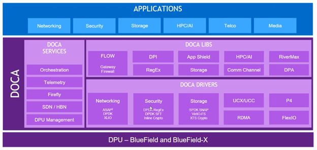
 NVIDIA Holoscan for HPC brings AI to edge computing. Streaming Reactive Framework will be released in June to simplify code changes to stream AI for instrument processing workflows.
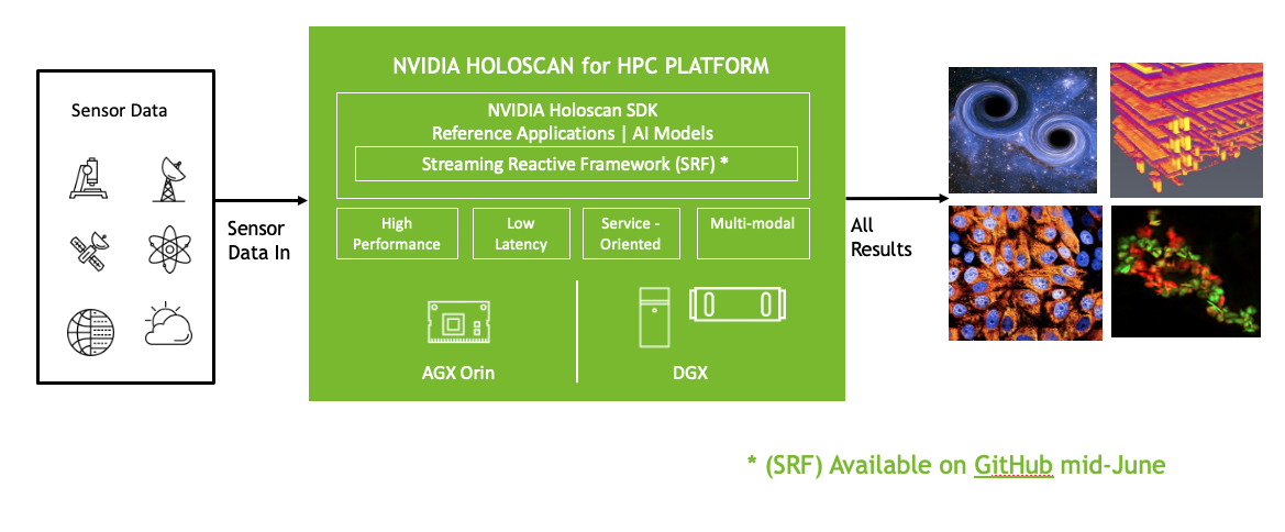
 Join this webinar on June 7 to learn how Aria Cybersecurity and NVIDIA are stopping modern security attacks in real time at demanding network speeds.

 Using Numba and PyOptiX, NVIIDA enables you to configure ray tracing pipeline and write kernels in Python compatible with the OptiX pipeline.
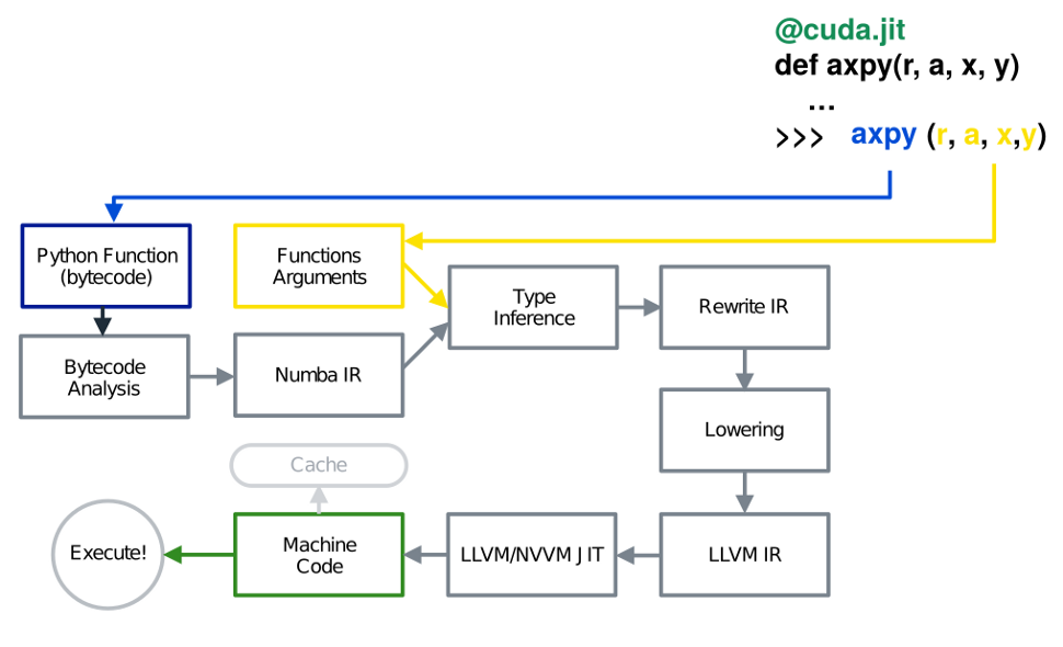