
Generative AI’s transformative effect on the auto industry took center stage last week at the International Motor Show Germany, known as IAA, in Munich. NVIDIA’s Danny Shapiro, VP of automotive marketing, explained in his IAA keynote how this driving force is accelerating innovation and streamlining processes — from advancing design, engineering and digital-twin deployment for Read article >
Category: Misc
 Spear phishing is the largest and most costly form of cyber threat, with an estimated 300,000 reported victims in 2021 representing $44 million in reported…
Spear phishing is the largest and most costly form of cyber threat, with an estimated 300,000 reported victims in 2021 representing $44 million in reported losses in the United States alone. Business e-mail compromises led to $2.4 billion in costs in 2021, according to the FBI Internet Crime Report. In the period from June 2016 to December 2021, costs related to phishing and spear phishing totaled $43 billion for businesses, according to IBM Security Cost of a Data Breach.
Spear phishing e-mails are indistinguishable from a benign e-mail that a victim would receive. This is also why traditional classification of spear phishing e-mails is so difficult. The content difference between a scam and a legitimate e-mail can be minuscule. Often, the only difference between the two is the intent of the sender: is the invoice legitimate, or is it a scam?
This post details a two-fold approach to improve spear phishing detection by boosting the signals of intent using NVIDIA Morpheus to run data processing and inferencing.
Generating e-mails with new phishing intent
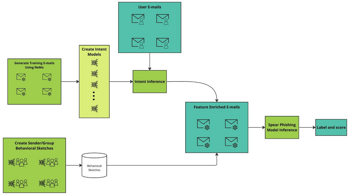
The first step involves using generative AI to create large, varied corpora of e-mails with various intents associated with spear phishing and scams. As new threats emerge, the NVIDIA Morpheus team uses the NVIDIA NeMo framework to generate a new corpus of e-mails with such threats. Following the generation of new e-mails with the new type of phishing intent, the team trains a new language model to recognize the intent. In traditional phishing detection mechanisms, such models would require a significant number of human-labeled e-mails.
Detecting sender intent
The first step targets the intent behind the e-mail. The next step targets the intent of the sender. To defend against spear phishing attacks that use spoofing, known senders, or longer cons that do not express their true intent immediately, we construct additional signals by building up behavioral sketches from senders or groups of senders.
Building on the intent work described above, known senders’ past observed intents are recorded. For example, the first time a known sender asks for money can be a signal to alert the user.
Syntax usage is also observed and recorded. The syntax of new e-mails is compared to the syntax history of the sender. A deviation from the observed syntax could indicate a possible spoofing attack.
Finally, the temporal patterns of a sender’s e-mails are collected and cross-referenced when a new e-mail arrives to check for out-of-pattern behavior. Is the sender sending an e-mail for the first time at midnight on a Saturday? If so, that becomes a signal in the final prediction. These signals in aggregate are used to classify e-mails. They are also presented to the end user as an explanation for why an e-mail may be malicious.
Adapting to new attacks and improving protection
Existing machine learning (ML) methods rely nearly entirely on human-labeled data and cannot adapt to emerging threats quickly. The biggest benefit to detecting spear phishing e-mails using the approach presented here is how quickly the model can be adapted to new attacks. When a new attack emerges, generative AI is leveraged to create a training corpus for the attack. Intent models are trained to detect its presence in received e-mails.
Using models built with NeMo generates thousands of high-quality, on-topic e-mails in just a few hours. The new intents are added to the existing spear phishing detector. The entire end-to-end workflow of creating new phishing attack e-mails and updating the existing models happens in less than 24 hours. Once the models are in place, e-mail processing and inferencing become a Morpheus pipeline to provide near real-time protection against spear phishing threats.
Results
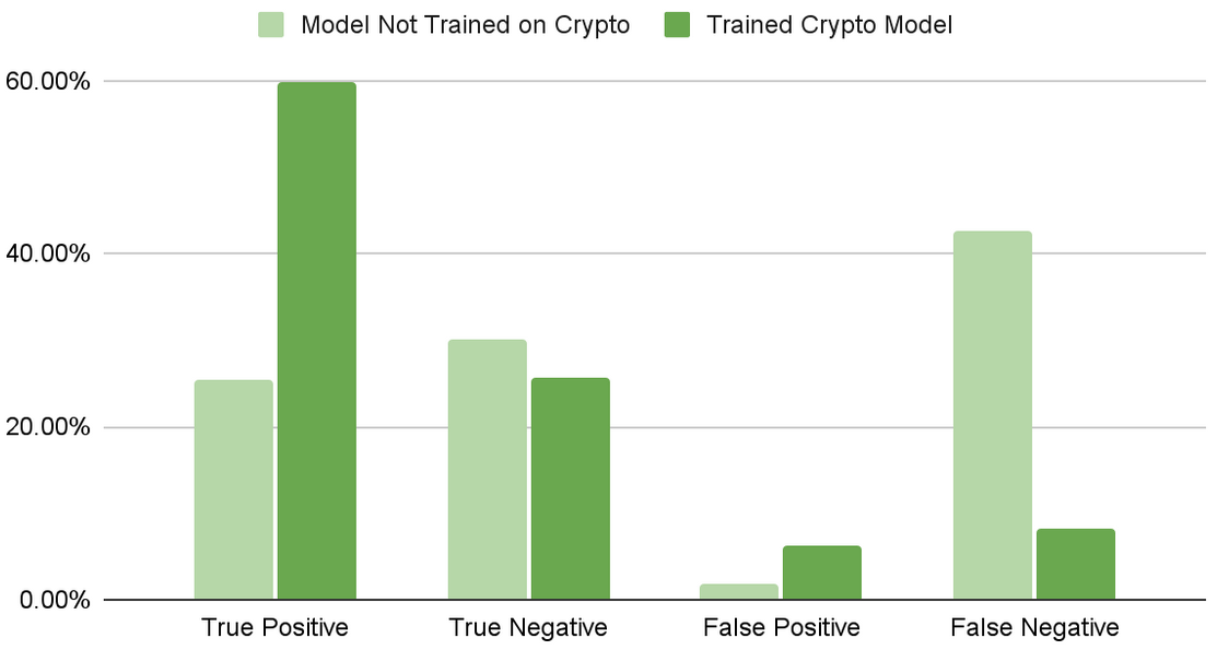
To illustrate the flexibility of this approach, a model was trained using only money, banking, and personal identifying information (PII) intents. Next, cryptocurrency-flavored phishing e-mails were generated using models built with NeMo. These e-mails were incorporated into the original training and validation subsets.
The validation set, now containing the new crypto attacks, was then passed into the original model. Then a second model was trained incorporating the crypto attack intents. Figure 2 shows how the models compare in their detection.
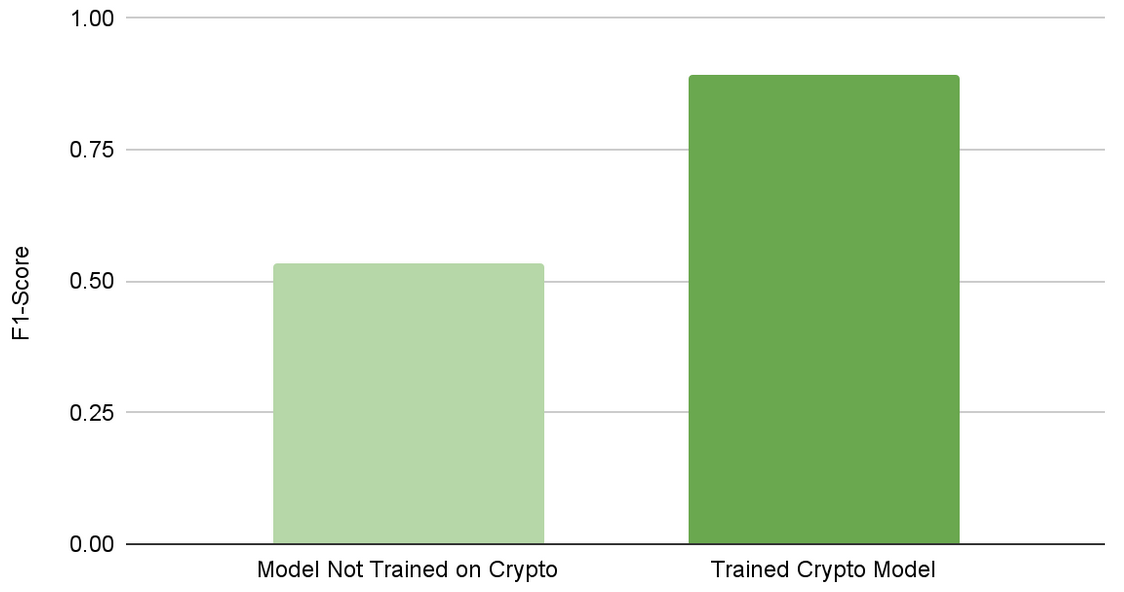
After training for the attack, the F1 score increased from 0.54 to 0.89 (Figure 3). This illustrates how quickly new attacks can be trained for and adapted to using NVIDIA Morpheus and NeMo.
Get started with NVIDIA Morpheus
Watch the video, Improve Spear Phishing Detection with Generative AI for more details. Learn more about how to use NVIDIA Morpheus to detect spear phishing e-mails faster and with greater accuracy using the NVIDIA AI workflow example. You can also apply to try NVIDIA Morpheus in LaunchPad and request a 90-day free trial to test drive NVIDIA Morpheus, part of the NVIDIA AI Enterprise software family.
 On Sept. 27, join us to learn recommender systems best practices for building, training, and deploying at any scale.
On Sept. 27, join us to learn recommender systems best practices for building, training, and deploying at any scale.
Ten miles in from Long Island’s Atlantic coast, Shinjae Yoo is revving his engine. The computational scientist and machine learning group lead at the U.S. Department of Energy’s Brookhaven National Laboratory is one of many researchers gearing up to run quantum computing simulations on a supercomputer for the first time, thanks to new software. Yoo’s Read article >
 The camera module is the most integral part of an AI-based embedded system. With so many camera module choices on the market, the selection process may seem…
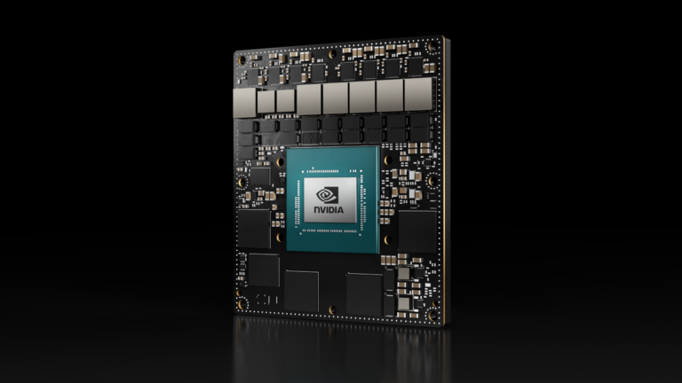
The camera module is the most integral part of an AI-based embedded system. With so many camera module choices on the market, the selection process may seem overwhelming. This post breaks down the process to help make the right selection for an embedded application, including the NVIDIA Jetson.
Camera selection considerations
Camera module selection involves consideration of three key aspects: sensor, interface (connector), and optics.
Sensor
The two main types of electronic image sensors are the charge-coupled device (CCD) and the active-pixel sensor (CMOS). For a CCD sensor, pixel values can only be read on a per-row basis. Each row of pixels is shifted, one by one, into a readout register. For a CMOS sensor, each pixel can be read individually and in parallel.
CMOS is less expensive and consumes less energy without sacrificing image quality, in most cases. It can also achieve higher frame rates due to the parallel readout of pixel values. However, there are some specific scenarios in which CCD sensors still prevail—for example, when long exposure is necessary and very low-noise images are required, such as in astronomy.
Electronic shutter
There are two options for the electronic shutter: global or rolling. A global shutter exposes each pixel to incoming light at the same time. A rolling shutter exposes the pixel rows in a certain order (top to bottom, for example) and can cause distortion (Figure 1).
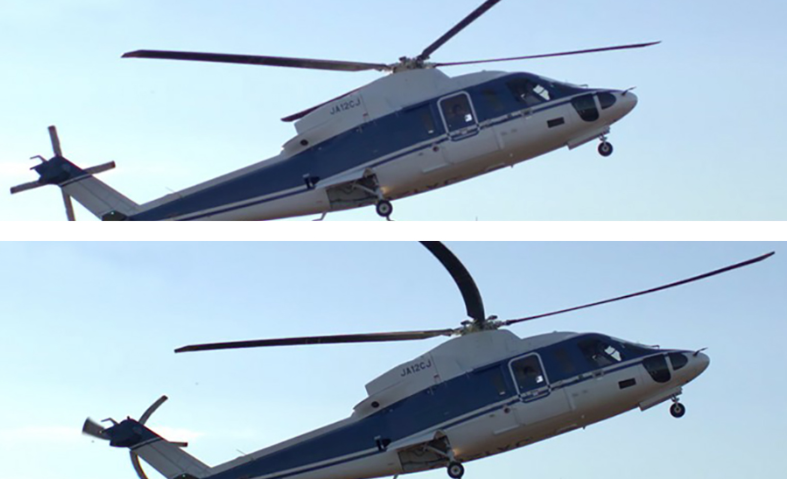
The global shutter is not impacted by motion blur and distortion due to object movement. It is much easier to sync multiple cameras with a global shutter because there is a single point in time when exposure starts. However, sensors with a global shutter are much more expensive than those with a rolling shutter.
Color or monochrome
In most cases, a monochrome image sensor is sufficient for typical machine vision tasks like fault detection, presence monitoring, and recording measurements.
With a monochrome sensor, each pixel is usually described by eight bits. With a color sensor, each pixel has eight bits for the red channel, eight bits for the green channel, and eight bits for the blue channel. The color sensor requires processing three times the amount of data, resulting in a higher processing time and, consequently, a slower frame rate.
Dynamic range
Dynamic range is the ratio between the maximum and minimum signal that is acquired by the sensor. At the upper limit, pixels appear white for higher values of intensity (saturation), while pixels appear black at the lower limit and below. An HDR of at least 80db is needed for indoor application and up to 140db is needed for outdoor application.
Resolution
Resolution is a sensor’s ability to reproduce object details. It can be influenced by factors such as the type of lighting used, the sensor pixel size, and the capabilities of the optics. The smaller the object detail, the higher the required resolution.
Pixel resolution translates to how many millimeters each pixel is equal to on the image. The higher the resolution, the sharper your image will be. The camera or sensor’s resolution should enable coverage of a feature’s area of at least two pixels.
CMOS sensors with high resolutions tend to have low frame rates. While a sensor may achieve the resolution you need, it will not capture the quality images you need without achieving enough frames per second. It is important to evaluate the speed of the sensor.
A general rule of thumb to determine the resolution needed for the use case is shown below and in Figure 2. The multiplier (2) represents the typical desire to have a minimum two pixels on an object in order to successfully detect it.

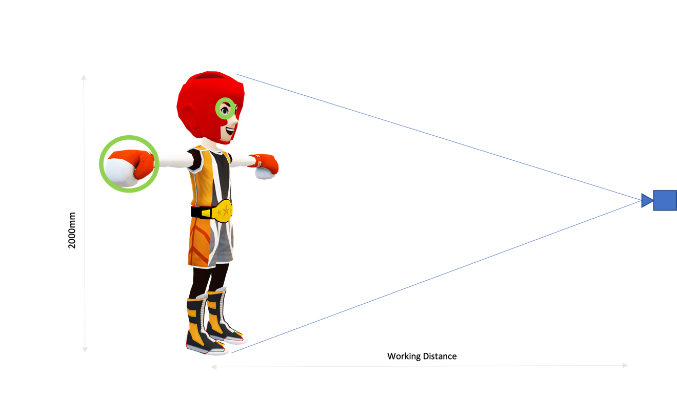
For example, suppose you have an image of an injury around the eye of a boxer.
- FOV, mm = 2000mm
- Size of feature of interest (the eye), mm = 4mm

Based on the calculation, 1000 x 1000, a one-megapixel camera should be sufficient to detect the eye using a CV or AI algorithm.
Note that a sensor is made up of multiple rows of pixels. These pixels are also called photosites. The number of photons collected by a pixel is directly proportional to the size of the pixel. Selecting a larger pixel may seem tempting but may not be the optimal choice in all the cases.
| Small pixel | Sensitive to noise (-) | Higher spatial resolution for same sensor size (+) |
| Large pixel | Less sensitive to noise (+) | Less spatial resolution for same sensor size (-) |
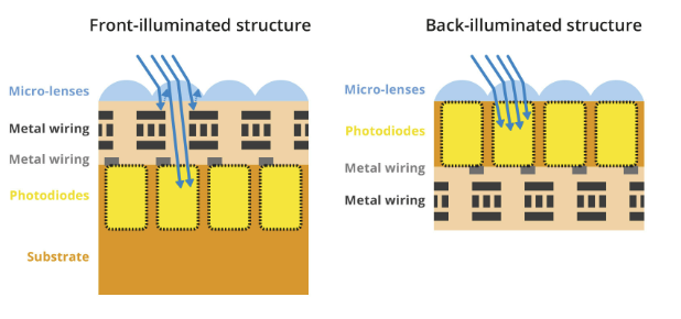
Back-illuminated sensors maximize the amount of light being captured and converted by each photodiode. In front-illuminated sensors, metal wiring above the photodiodes blocks off some photons, hence reducing the amount of light captured.
Frame rate and shutter speed
The frame rate refers to the number of frames (or images captured) per second (FPS). The frame rate should be determined based on the number of inspections required per second. This correlates with the shutter speed (or exposure time), which is the time that the camera sensor is exposed to capture the image.
Theoretically, the maximum frame rate is equal to the inverse of the exposure time. But achievable FPS is lower because of latency introduced by frame readout, sensor resolution, and the data transfer rate of the interface including cabling.
FPS can be increased by reducing the need for large exposure times by adding additional lighting, binning the pixels.
CMOS sensors can achieve higher FPS, as the process of reading out each pixel can be done more quickly than with the charge transfer in a CCD sensor’s shift register.
Interface
There are multiple ways to connect the camera module to an embedded system. Typically, for evaluation purposes, cameras with USB and Ethernet interfaces are used because custom driver development is not needed.
Other important parameters for interface selection are transmission length, data rate, and operating conditions. Table 2 lists the most popular interfaces. Each option has its pros and cons.
| Features | USB 3.2 | Ethernet (1 GbE) | MIPI CSI-2 | GMSL2 | FPDLINK III |
| Bandwidth | 10Gbps | 1Gbps | DPHY 2.5 Gbps/lane CPHY 5.71 Gbps/lane | 6Gbps | 4.2Gbps |
| Cable length supported | Up to 100m | ||||
| Plug-and-play | Supported | Supported | Not supported | Not supported | Not supported |
| Development costs | Low | Low | Medium to high | Medium to high | Medium to high |
| Operating environment | Indoor | Indoor | Indoor | Indoor and outdoor | Indoor and outdoor |
Optics
The basic purpose of an optical lens is to collect the light scattered by an object and recreate an image of the object on a light-sensitive image sensor (CCD or CMOS). The following factors should be considered when selecting an optimized lens-focal length, sensor format, field of view, aperture, chief ray angle, resolving power, and distortion.
Lenses are manufactured with a limited number of standard focal lengths. Common lens focal lengths include 6mm, 8mm, 12.5mm, 25mm, and 50mm.
Once you choose a lens with a focal length closest to the focal length required by your imaging system, you need to adjust the working distance to get the object under inspection in focus. Lenses with short focal lengths (less than 12mm) produce images with a significant amount of distortion.
If your application is sensitive to image distortion, try to increase the working distance and use a lens with a higher focal length. If you cannot change the working distance, you are somewhat limited in choosing an optimized lens.
| Wide-angle lens | Normal lens | Telephoto lens | |
| Focal length | 50mm | >=70mm | |
| Use case | Nearby scenes | Same as human eye | Far-away scenes |
To attach a lens to a camera requires some type of mounting system. Both mechanical stability (a loose lens will deliver an out-of-focus image) and the distance to the sensor must be defined.
To ensure compatibility between different lenses and cameras, the following standard lens mounts are defined.
| Most popular | For industrial applications | |
| Lens mount | M12/S mount | C-mount |
| Flange focal length | Non-standard | 17.526mm |
| Threads (per mm) | 0.5 | 0.75 |
| Sensor size accommodated (inches) | Up to ⅔ | Up to 1 |
NVIDIA camera module partners
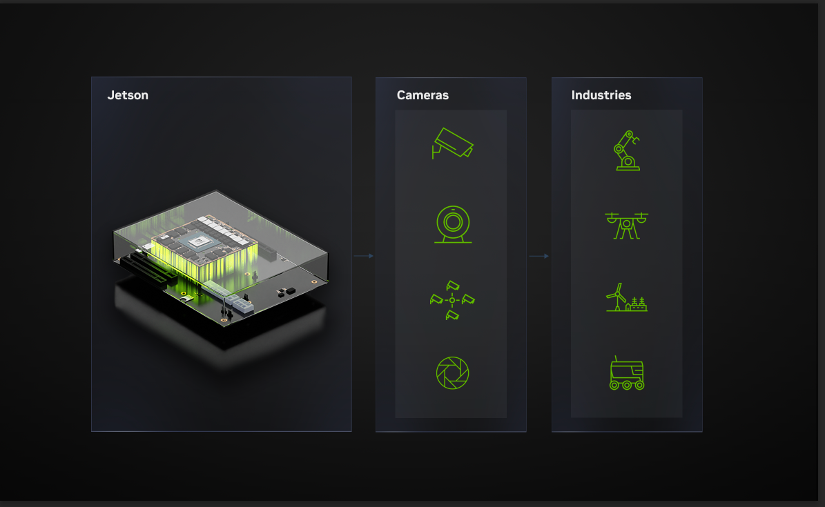
NVIDIA maintains a rich ecosystem of partnerships with highly competent camera module makers all over the world. See Jetson Partner Supported Cameras for details. These partners can help you design imaging systems for your application from concept to production for the NVIDIA Jetson.
Summary
This post has explained the most important camera characteristics to consider when selecting a camera for an embedded application. Although the selection process may seem daunting, the first step is to understand your key constraints based on design, performance, environment, and cost.
Once you understand the constraints, then focus on the characteristics most relevant to your use case. For example, if the camera will be deployed away from the compute or in a rugged environment, consider using the GMSL interface. If the camera will be used in low-light conditions, consider a camera module with larger pixel and sensor sizes. If the camera will be used in a motion application, consider using a camera with a global shutter.
To learn more, watch Optimize Your Edge Application: Unveiling the Right Combination of Jetson Processors and Cameras. For detailed specs on AI performance, GPU, CPU, and more for both Xavier and Orin-based Jetson modules, visit Jetson Modules.
Editor’s note: This post is part of our weekly In the NVIDIA Studio series, which celebrates featured artists, offers creative tips and tricks and demonstrates how NVIDIA Studio technology improves creative workflows. When it comes to converting 2D concepts into 3D masterpieces, self-taught visual development artist Alex Treviño has confidence in the potential of all Read article >
 Explore how ray-traced caustics combined with NVIDIA RTX features can enhance the performance of your games.
Explore how ray-traced caustics combined with NVIDIA RTX features can enhance the performance of your games.
In its debut on the MLPerf industry benchmarks, the NVIDIA GH200 Grace Hopper Superchip ran all data center inference tests, extending the leading performance of NVIDIA H100 Tensor Core GPUs. The overall results showed the exceptional performance and versatility of the NVIDIA AI platform from the cloud to the network’s edge. Separately, NVIDIA announced inference Read article >
 The first post in this series introduced vector search indexes, explained the role they play in enabling a widespread range of important applications, and…
The first post in this series introduced vector search indexes, explained the role they play in enabling a widespread range of important applications, and provided a brief overview of vector search on the GPU with the RAFT library.
In this post, we dive deeper into each of the GPU-accelerated indexes mentioned in Part 1 and give a brief explanation of how the algorithms work, along with a summary of important parameters to fine-tune their behavior.
We then go through a simple end-to-end example to demonstrate RAFT’s Python APIs on a question-and-answer problem with a pretrained large language model and provide a performance comparison of RAFT’s algorithms against HNSW for a few different scenarios involving different numbers of query vectors being passed to the search algorithm concurrently.
This post provides:
- An overview of vector search index algorithms that can be used with GPUs
- An end-to-end example demonstrating how easy it can be to run vector search on the GPU with Python
- Performance comparison of vector search on the GPU against HNSW, the current state-of-the-art method on the CPU
Vector search indexes
When working with vector search, the vectors are often converted to an indexed format that is optimized for fast lookups. Choosing the right indexing algorithm is important as it can affect both index build and search times. Furthermore, each different index type comes with its own set of knobs for fine-tuning the behavior, trading off index construction time, storage cost, search quality, and search speed.
When the right indexing algorithm is paired with the correct parameter settings, vector search on the GPU provides both faster build and search times for all levels of recall.
IVF-Flat
As it’s the simplest index type, start with the IVF-Flat algorithm. In this algorithm, a set of training vectors are first split into some clusters and then stored in the GPU memory organized by their closest cluster centers. The index-building step is faster than that of other algorithms presented in this post, even at high numbers of clusters.
To search an IVF-Flat index, the closest clusters to each query vector are selected, and the k-nearest neighbors (k-NN) are computed from each of those closest clusters. Because IVF-Flat stores the vectors in an exact, or flat format, meaning without compression, it has the advantage of computing exact distances within each of the clusters it searches. As we describe later in this post, this provides an advantage that often has a higher recall than IVF-PQ when the same number of closest clusters are searched. IVF-Flat index is a good choice when the full index can fit in GPU memory.
RAFT’s IVF-Flat index contains a couple of parameters to help trade off the query performance and accuracy:
- When training the index, the
n_listsparameter determines the number of clusters to partition the training dataset. - The search parameter
n_probesdetermines the number of closest clusters to search through to compute the nearest neighbors for a set of query points.
In general, a smaller number of probes leads to a faster search at the expense of recall. When the number of probes is set to the number of lists, exact results are computed. However, in that case, a call to RAFT’s brute-force search is more performant.
IVF-PQ
When your dataset becomes too large to fit on the GPU, you gain some mileage by compressing the vectors using the IVF-PQ index type. Like IVF-Flat, IVF-PQ splits the points into a number of clusters (also specified by a parameter called n_lists) and searches the closest clusters to compute the nearest neighbors (also specified by a parameter called n_probes), but it shrinks the sizes of the vectors using a technique called product quantization.
Compressing the index ultimately allows for more vectors to be stored on the GPU. The amount of compression can be controlled with tuning parameters, which we describe later in this post, but higher levels of compression can provide a faster lookup time at the cost of recall. IVF-PQ is currently RAFT’s most memory-efficient vector index.
RAFT’s IVF-PQ provides two parameters that control memory usage:
pq_dimsets the target dimensionality of the compressed vector.pq_bitssets the number of bits for each vector element after compression.
We recommend setting the former to a multiple of 32 while the latter is limited to a range of 4-8 bits. By default, RAFT selects a dimensionality value that minimizes quantization loss according to pq_bits, but this value can be adjusted to lower the memory footprint for each vector. It is useful to play with these parameters to see which settings work best for you.
When using large amounts of compression, an additional refinement step can be performed by querying the IVF-PQ index for a larger number of neighbors than needed and computing an exact search over the resulting neighbors to reduce the set down to the final desired number. The refinement step requires the original uncompressed dataset on the host memory.
For more information about building an IVF-PQ index, with in-depth details and recommendations, see the complete guide to RAFT IVF-PQ notebook on our GitHub repo.
CAGRA
CAGRA is RAFT’s new state-of-the-art ANN index. It is a high-performance, GPU-accelerated, graph-based method that has been specifically optimized for small-batch cases, where each lookup contains only one or a few query vectors. Like other popular graph-based methods, such as hierarchical navigable small-world graphs (HNSW) and SONG, an optimized k-NN graph is built at index training time with various qualities that yield efficient search at reasonable levels of recall.
CAGRA performs a search by first randomly selecting candidate vertices from the graph and then expanding, or traversing, those vertices to compute distances to their children, storing off the nearest neighbors along the way (Figure 1). Each time it traverses a set of vertices, it has performed one iteration.
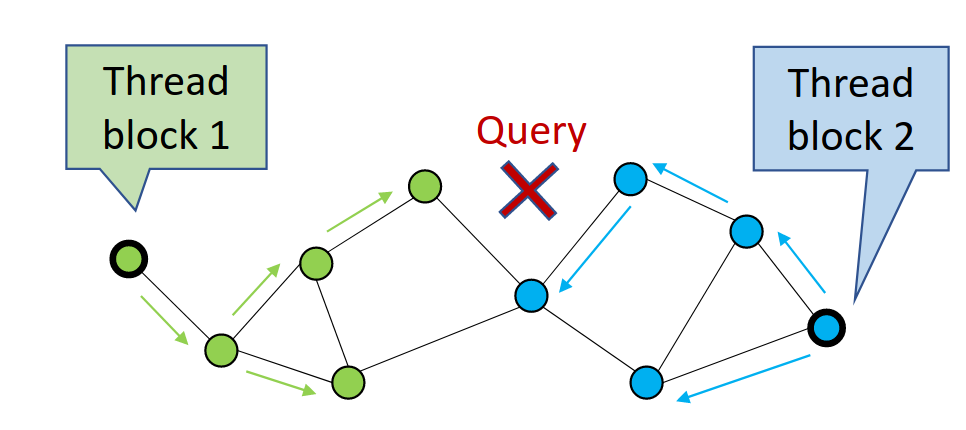
In Figure 1, CAGRA is using multiple thread blocks to visit more graph nodes in parallel. This is maximizing GPU utilization for single-query searches.
Because CAGRA returns the approximate nearest neighbors like the algorithms described earlier, it also provides a few parameters to control the recall and the speed.
The main parameter that can be adjusted to trade off search speed is itopk_size, which specifies the size of an internal sorted list that stores the nodes that can be explored in the next iteration. Higher values of itopk_size keep a larger search context in memory that improves recall at the cost of more time spent in maintaining the queue.
The parameter search_width defines the number of the closest parent vertices that are traversed to expand their children in each search iteration.
Another useful parameter is the number of iterations to perform. The setting is selected automatically by default, but this can be changed to a higher or lower value to trade off recall for a faster search.
CAGRA’s optimized graph is fixed-degree, which is tuned using the parameter graph_degree. The fixed-degree makes better use of GPU resources by keeping the number of computations uniform when searching the graph. It builds the initial k-NN graph by computing an actual k-NN, for example by using IVF-PQ explained earlier, to compute the nearest neighbors of all the points in the training dataset.
The number of k-nearest neighbors (k) of this intermediate k-NN graph can be tuned using a parameter called intermediate_graph_degree to trade off the quality of the final searchable CAGRA graph.
A higher quality graph can be built with a larger intermediate_graph_degree value, which means that the final optimized graph is more likely to find nearest neighbors that yield a high recall. RAFT provides several useful parameters to tune the CAGRA algorithm. For more information, see the CAGRA API documentation.
Again, this parameter can be used to control how thoroughly the overall space is covered by the search but again this comes at the cost of having to search more to find the nearest neighbors, which reduces the search performance.
Getting started with pylibraft
Pylibraft is the lightweight Python library of RAFT and enables you to use RAFT’s ANN algorithms for vector search right in Python. Pylibraft can accept any object that supports __cuda_array_interface__, such as a Torch or CuPy array.
The following example briefly demonstrates how you can build and query a RAFT CAGRA index with Pylibraft.
from pylibraft.neighbors import cagra
import cupy as cp

# On small batch sizes, using "multi_cta" algorithm is efficient
index_params = cagra.IndexParams(graph_degree=32)
search_params = cagra.SearchParams(algo="multi_cta")

corpus_embeddings = cp.random.random((1500,96), dtype=cp.float32)
query_embeddings = cp.random.random((1,96), dtype=cp.float32)

cagra_index = cagra.build(index_params, corpus_embeddings)
# Find the 10 closest vectors
hits = cagra.search(search_params, cagra_index, query_embeddings, k=10)
With the recent success of LLMs, semantic search is a perfect way to showcase vector similarity search in action using RAFT. In the following example, a DistilBERT transformer model combined with each of the three ANN indexes is used to solve a simple question retrieval problem. The Simple English Wikipedia dataset is used to answer the user’s search query.
The language model first transforms the training sentences into vector embeddings that are inserted into a RAFT ANN index. The inference is done by encoding the query and using our trained ANN index to find vectors similar to the encoded query vector. The answer that you return to the user is the nearest article in Simple Wikipedia, which you fetch using the closest vector from the similarity search.
You can get started with RAFT by using pylibraft and this notebook for a question-retrieval task:
Sorry, something went wrong. Reload?
Sorry, we cannot display this file.
Sorry, this file is invalid so it cannot be displayed.
Viewer requires iframe.
Benchmarks
Using GPU as a hardware accelerator for your vector search application can lead to an increase in performance, and it is best showcased on large datasets. The benchmarks can be fully reproduced by following RAFT’s end-to-end benchmark documentation. Our benchmarks consider that the data is already available for computation, which means that data transfer is not taken into consideration, although this should not be a significant difference thanks to the high transfer speed of recent NVIDIA hardware (over 25 GB/s).
We used the DEEP-100M dataset on an H100 GPU to compare RAFT indexes with HNSW running on an Intel Xeon Platinum 8480CL CPU.
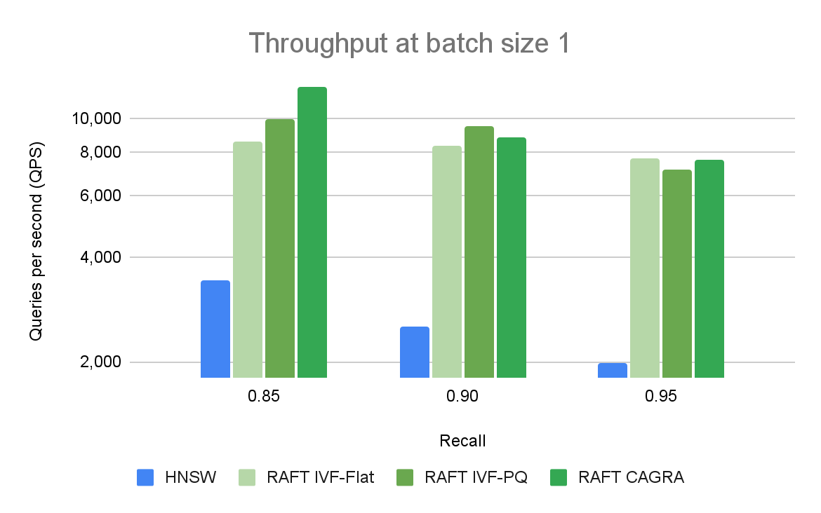
Figure 2 compares ANN algorithms at various levels of recall and throughput for a single query. At high levels of recall, RAFT’s methods demonstrate higher throughput than other alternative libraries.
We ran a performance comparison on queries for a single vector at a time, called online search. It’s one of the main use cases for vector search. RAFT-based indexes provide a higher throughput, measured in queries-per-second (QPS), than other libraries that are using CPU or GPU.
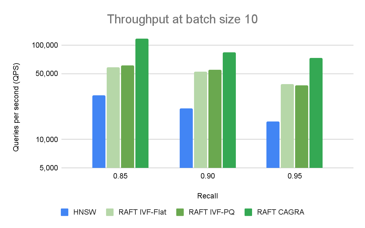
Figure 3 compares ANN algorithms at various levels of recall and throughput with a batch size of 10 queries. RAFT’s methods demonstrate higher throughput than HNSW for all experiments.
The benefits of using GPU for vector search applications are most prevalent at higher batch sizes. The performance gap between CPU and GPU is significant and can scale up easily. Figure 3 shows that for a batch size of 10, only RAFT-based indexes are relevant when comparing the number of queries per second. For a batch size of 10k (Figure 4), CAGRA outperforms all other indexes by far.
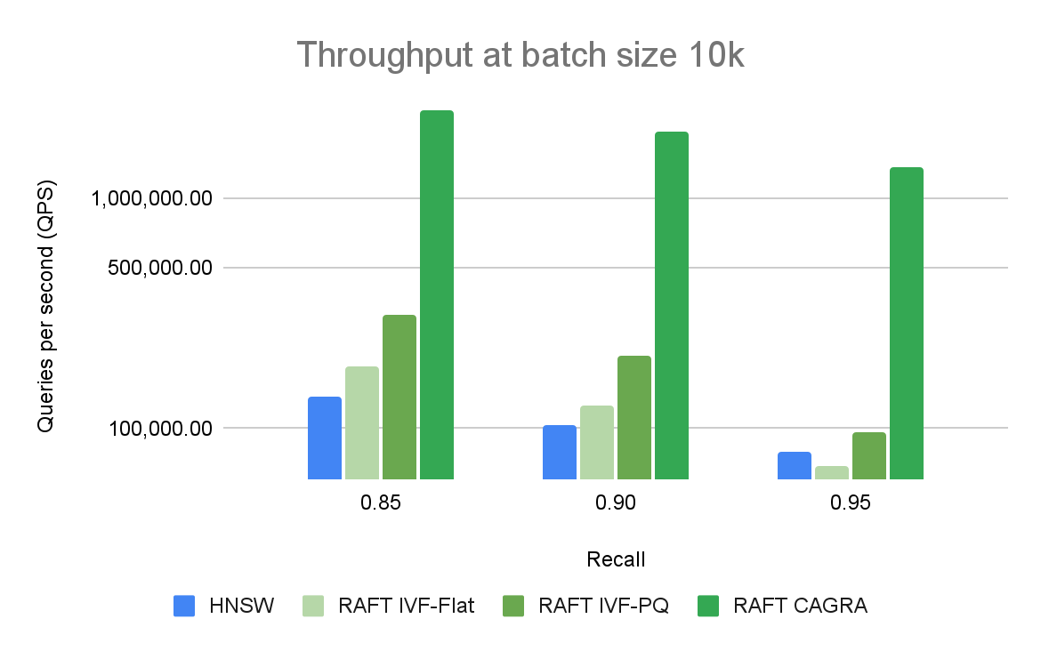
Figure 4 compares ANN algorithms at various levels of recall and throughput with a batch size of 10K query. RAFT’s methods demonstrate higher throughput than HNSW for all experiments.
Summary
Each different vector search index type has benefits and drawbacks which ultimately depend on your needs. This post outlined some of those benefits and drawbacks, providing a brief explanation of how each different algorithm works, along with a few of the most important parameters that can be tuned to trade off storage costs, build times, search quality, and search performance. In all cases, GPUs can improve both index construction and search performance.
RAPIDS RAFT is fully open source and available on the /rapidsai/raft GitHub repo. You can get started with RAFT by reading through the docs, running the reproducible benchmarking suite, or building upon the example vector search template project. Also be sure to look for options to enable RAFT indexes in Milvus, Redis, and FAISS. Finally, you can follow us on Twitter at @rapidsai.
 In the AI landscape of 2023, vector search is one of the hottest topics due to its applications in large language models (LLM) and generative AI. Semantic…
In the AI landscape of 2023, vector search is one of the hottest topics due to its applications in large language models (LLM) and generative AI. Semantic vector search enables a broad range of important tasks like detecting fraudulent transactions, recommending products to users, using contextual information to augment full-text searches, and finding actors that pose potential security risks.
Data volumes continue to soar and traditional methods for comparing items one by one have become computationally infeasible. Vector search methods use approximate lookups, which are more scalable and can handle massive amounts of data more efficiently. As we show in this post, accelerating vector search on the GPU provides not only faster search times, but the index building times can also be substantially faster.
This post provides:
- An introduction to vector search with a brief review of popular applications
- An overview of the RAFT library for accelerating vector search on the GPU
- Performance comparison of GPU-accelerated vectors search indexes against the state-of-the-art on the CPU
The second post in this series dives deeper into each of the GPU-accelerated indexes mentioned in this post and gives a brief explanation of how the algorithms work, along with a summary of important parameters to fine-tune their behavior. For more information, see Accelerating Vector Search: Fine-Tuning GPU Index Algorithms.
What is vector search?
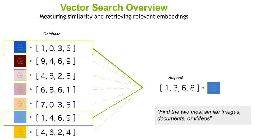
Figure 1 shows that vector search entails creating an index of vectors and performing lookups to find some number of vectors in the index that are closest to a query vector. The vectors could be as small as three-dimensional points from a lidar point cloud or larger embeddings from text documents, images, or videos.
Vector search is the process of querying a database to find the most similar vectors. This similarity search is done on numerical vectors that can represent any type of object (Figure 2). These vectors are often embeddings created from multimedia like images, video, and text fragments or entire documents that went through a deep learning model to encode their semantic characteristics into a vector form.
Embedding vectors typically have the advantage of being a smaller object than the original document (lower dimensionality), while maintaining as much information about the source as possible. Therefore, two documents that are similar often have similar embeddings.
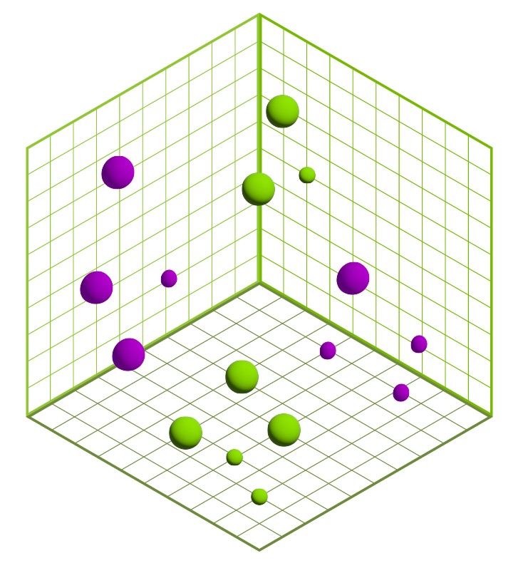
The points in Figure 2 are 3D but they could be 500 dimensions or even higher.
This makes it easier to compare objects, as the embedding vectors are smaller and retain most of the information. When two documents share similar characteristics, their embedding vectors are often spatially close, or similar.
Approximate methods for vector search
To handle larger datasets efficiently, approximate nearest neighbor (ANN) methods are often used for vector search. ANN methods speed up the search by approximating the closest vectors. This avoids the exhaustive distance computation often required by an exact brute-force approach, which requires comparing the query against every single vector in the database.
In addition to the search compute cost, storing many vectors can also consume a large amount of memory. To ensure both fast searches and low memory usage, you must index vectors in an efficient way. As we outline a bit later, this can sometimes benefit from compression. A vector index is a space-efficient data structure built on mathematical models that is used for efficiently querying several vectors at a time.
Updating the indexes, such as from inserting and deleting vectors, can cause problems when indexes take hours or even days to build. It turns out that these indexes can often be built much faster on the GPU. We showcase this performance later in the post.
Vector search in LLMs
LLMs have become popular for capturing and preserving the semantic meaning and context of the original documents. This means that the vectors resulting from LLM models can be searched using vector similarity search. This search finds items that happen to contain similar words, shapes, or moving objects. It also finds vectors that contextually and semantically mean similar things.
This semantic search doesn’t rely on exact word matching. For example, searching for the term, “I would like to buy a muscle car” in an image database should be able to contextualize the sentence to understand the following:
- Buying a car is different from renting a car, so you’d expect to find vectors closer to car dealerships and reviews from car purchasers, rather than car rental companies.
- A muscle car is different from a bodybuilder so you’d expect to find vectors about Dodge Chargers and not Arnold Schwarzenegger.
- Buying a muscle car is different from buying muscle relaxers or economy vehicles.
More recently, large language transformer-based models like ChatGPT, LLaMa, NeMo, and BERT have provided significant technical leaps that are increasing the contextual awareness of the models and making them even more useful and applicable to more industries.
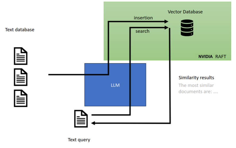
In addition to creating embedding vectors that can be stored and later searched, these new LLM models use semantic search in pipelines that generate new content from context gleaned by finding similar vectors. This content generation process, shown in Figure 3, is known as retrieval-augmented generative AI.
Using vector search in a vector database
A vector database stores high-dimensional vectors (for example, embeddings), and facilitates fast and accurate search and retrieval based on vector similarity (for example, ANN algorithms). Some databases are purpose-built for vector search (for example, Milvus). Other databases include vector search capabilities as an additional feature (for example, Redis).
Choosing which vector database to use depends on the requirements of your workflow.
Retrieval-augmented language models allow pretrained models to be customized for specific products, services, or other domain-specific use cases by augmenting a search with additional context that has been encoded into vectors by the LLM and stored in a vector database.
More specifically, a search is encoded into vector form and similar vectors are found in the vector database to augment the search. The vectors are then used with the LLM to formulate an appropriate response. Retrieval-augmented LLMs are a form of generative AI and they have revolutionized the industry of chatbots and semantic text search.
Other applications of vector similarity search
In addition to retrieval-augmented LLMs for generative AI, vector embeddings have been around for some time and have found many useful applications in the real world:
- Recommender systems: Provide personalized suggestions according to what a user has shown interest in or interacted with.
- Finance: Fraud detection models vectorize user transactions, making it possible to determine whether those transactions are similar to typical fraudulent activities.
- Cybersecurity: Uses embeddings to model and search behaviors of bad actors and anomalous activities.
- Genomics: Finds similar genes and cell structures in genomics analysis, such as single-cell RNA analysis.
- Chemistry: Models molecular descriptors or fingerprints of chemical structures to compare them or find similar structures in a database.
We are always interested in learning about your use cases so don’t hesitate to leave a comment if you either use vector search already or would like to discuss how it could benefit your application.
RAPIDS RAFT library for vector search
RAFT is a library of composable building blocks for accelerating machine learning algorithms on the GPU, such as those used in nearest neighbors and vector search. ANN algorithms are among the core building blocks that comprise vector search libraries. Most importantly, these algorithms can greatly benefit from GPU acceleration.
For more information about RAFT’s core APIs and the various accelerated building blocks that it contains, see Reusable Computational Patterns for Machine Learning and Data Analytics with RAPIDS RAFT.
ANN for fast searches
In addition to brute-force for exact search, RAFT currently provides three different algorithms for ANN search:
- IVF-Flat
- IVF-PQ
- CAGRA
The choice of the algorithm can depend upon your needs, as they each offer different advantages. Sometimes, brute force can even be the better option. More are being added in upcoming releases.
Because these algorithms are not doing an exact search, it is possible that some highly similar vectors are missed. The recall metric can be used to represent how many neighbors in the results are actual nearest neighbors of the query. Most of our benchmarks target recall levels of 85% and higher, meaning 85% (or more) of the relevant vectors were retrieved.
To tune the resulting indexes for different levels of recall, use various settings, or hyperparameters, when training approximate nearest-neighbors algorithms. Reducing the recall score often increases the speed of your searches and increasing the recall decreases the speed. This is known as the recall-speed tradeoff.
For more information, see Accelerating Vector Search: Fine-Tuning GPU Index Algorithms.
Performance comparison
GPUs excel at processing a lot of data at one time. All the algorithms just mentioned can outperform corresponding algorithms on the CPU when computing the nearest neighbors for thousands or tens of thousands of points at a time.
However, CAGRA was specifically engineered with online search in mind, which means that it outperforms the CPU even when only querying the nearest neighbors for a few data points at a time.
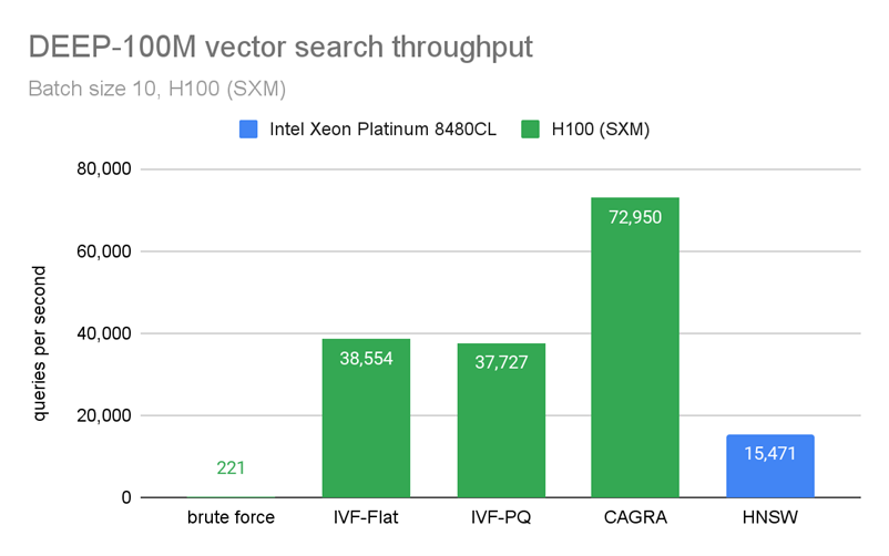
Figure 4 and Figure 5 show benchmarks that we performed by building an index on 100M vectors and querying only 10 vectors at a time. In Figure 4, CAGRA outperforms HNSW, which is one of the most popular indexes for vector search on CPU, in raw search performance even for an extremely small batch size of 10 vectors. This speed comes at a memory cost, however. In Figure 5, you can see that CAGRA’s memory footprint is a bit higher than the other nearest neighbors methods.
In Figure 5, the host memory of IVF-PQ is for the optional refinement step.
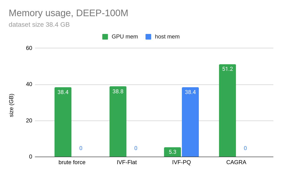
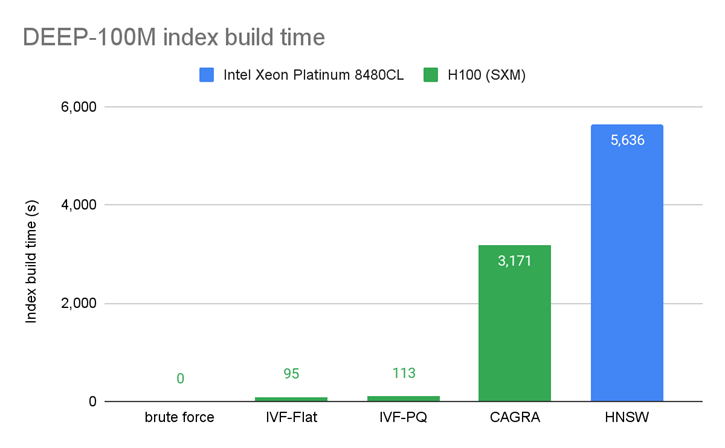
Figure 6 presents a comparison of the index build times and shows that indexes can often be built faster on the GPU.
Summary
From feature stores to generative AI, vector similarity search can be applied in every industry. Vector search on the GPU performs at lower latency and achieves higher throughput for every level of recall for both online and batch processing.
RAFT is a set of composable building blocks that can be used to accelerate vector search in any data source. It has pre-built APIs for Python and C++. Integration for RAFT is underway for Milvus, Redis, and FAISS. We encourage database providers to try RAFT and consider integrating it into their data sources.
In addition to state-of-the-art ANN algorithms, RAFT contains other GPU-accelerated building blocks, such as matrix and vector operations, iterative solvers, and clustering algorithms. The second post in this series dives deeper into each of the GPU-accelerated indexes mentioned in this post and gives a brief explanation of how the algorithms work, along with a summary of important parameters to fine-tune their behavior. For more information, see Accelerating Vector Search: Fine-Tuning GPU Index Algorithms.
RAPIDS RAFT is fully open source and available on the /rapidsai/raft GitHub repo. You can also follow us on Twitter at @rapidsai.