Hey guys, I know this may not be the perfect place, but I though some of you may have the skills and the interest to apply to some recent job openings. I you are not interested in these jobs just ignore them, downvote them, but there may be other who not only find them useful but they can make a difference if you are interested in them apply directly to the link, we are searching for North America based individuals (for tax reasons)only, thanks!
Spatiotemporal blue noise textures add the time axis, providing better convergence of blue noise, without loss of quality of the blue noise error patterns.
In the first post, Rendering in Real Time with Spatiotemporal Blue Noise, Part 1, we introduced the time axis and importance sampling to blue noise textures. In this post, we take a deeper look, show a few extensions, and explain some best practices.
Neighboring pixels in blue noise textures have very different values from each other, including wrap around neighbors, as if the texture were tiled. The assumption is that when you have a function that renders a pixel , small changes in x result in small changes in y, and that big changes in x result in big changes in y.
When you put very different neighbor values in for x, you also then get very different neighbor values out for y, tending to make the rendered result have blue noise error patterns. This assumption usually holds, unless your pixel rendering function is a hash function, on geometry edges, or on shading discontinuities.
It’s also worth noting that each pixel in spatiotemporal blue noise is a progressive blue noise sequence over time but is progressive from any point in the sequence. This can be seen when looking at the DFT and remembering that the Fourier transform assumes infinite repetition of the sequence being transformed.
There are no seams in the blue noise that would distort the frequency content. This means that when using TAA, where each pixel throws out its history on different timelines, every pixel is immediately on a good, progressive sampling sequence when rejecting history, instead of being on a less good sequence until the sequence restarts, as is common in other sampling strategies. In this way, each pixel in spatiotemporal blue noise is toroidally progressive.
It is worth mentioning is that that pixels under motion under TAA lose temporal benefits and our noise then functions as purely spatial blue noise. Pixels that are still even for a moment gain temporal stability and lower error, however, which is then carried around by TAA when they are in motion again. In these situations, our noise does no worse than spatial blue noise, so should always be used instead, to gain benefits where available and do no worse otherlwise.
Figure 1a. Convergence rate of ray traced AO when all pixels are still
Figure 1b. Convergence rate of ray traced AO when all pixels are in motion
Denoising blue noise
Blue noise is more easily removed from an image than white noise due to digital signal processing reasons. White noise has randomization in all frequencies, while blue noise has randomization only in high frequencies.
A blur, such as a box filter or a Gaussian blur, is a low-pass filter, which that means it removes high frequencies but enables low frequencies to remain.
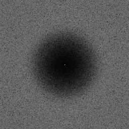
When white noise is blurred, it turns into noisy blobs, due to lower frequency randomization surviving the low-pass filter.
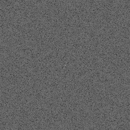
When blue noise is blurred, the high frequency noise goes away and leaves the lower frequencies of the image intact.
Blue noise uses Gaussian energy functions during its creation so it is optimized to be removed by Gaussian blurs. If you blur blue noise with a Gaussian function and are seeing noisy blobs remain, that means you must use a larger sigma in the blur, due to the lower frequencies of the blue noise passing through the filter. There may be a balance between removing those blobs and preserving more detail in the denoised image. It depends on your preferences.
Figures 2, 3, and 4 show how blue noise compares to white noise both when used raw, as well as when denoised.
Figure 2a. An 8-bit per color channel image.
Figure 2b. An image quantized to 1-bit per color channel using rounding.
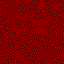
Figure 3a. White noise is used to dither before quantization, breaking up the banding into a noise pattern.
Figure 3b. Blue noise is used for the same, resulting in a better noise pattern.
In Figure 3, both images have only eight colors total, as they are only 1-bit per color channel. There are many more recognizable and finer details in the blue-noise–dithered image!
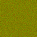
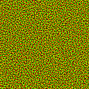
Figure 4a. The images from Figure 1 but put througha Gaussian blur. The white noise is still much more noticeable, as larger, low frequency blobs.
Figure 4b. The blue noise has nearly melted away completely and just looks as if the source 24-bit per pixel image was blurred, despite going down to 3-bits per pixel.
To see the reason why blue noise denoises so much better than white noise, look at them in frequency space. You apply a Gaussian blur through convolution, which is the same as a pixel-wise multiplication in frequency space.
If you multiply the blue noise frequencies by the Gaussian kernel frequencies, there will be nothing left, and it will be all black; the Gaussian blur removes the blue noise.
If you multiply the white noise frequencies by the Gaussian kernel frequencies, you end up with something in the shape of the Gaussian kernel frequencies (low frequencies), but they are randomized. These are the blobs left over after blurring white noise.
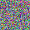
Figure 5 shows the frequency magnitudes of blue noise, white noise, and a Gaussian blur kernel.
Figure 5a. The frequencies present in blue noise
Figure 5b. The frequencies present in white noise
Figure 5c. The frequencies present in a Gaussian blur low pass filter.
Tiling blue noise
Blue noise tiles well due to not having any larger scale (lower frequency) content. Figure 6 shows how this is true but also shows that blue noise tiling gets more obvious at lower resolutions. This is important because blue noise textures are most commonly tiled across the screen and used in screen space. If you notice tiling when using blue noise, you should try a larger resolution blue noise texture.
Figure 6a. A 128×128 blue noise texture tiled 4×4 times
Figure 6b. A 16×16 blue noise texture tiled 32×32 times
Getting more than one value per pixel
There may be times you want more than one spatiotemporal blue noise value per pixel, like when rendering multiple samples per pixel.
One way to do this is to read the texture at some fixed offset. For instance, if you read the first value at (pixelX, pixelY) % textureSize, you might read the second value at (pixelX+5, pixelY+7) % textureSize. This essentially gives you an uncorrelated spatiotemporal blue noise value, just as if you had a second spatiotemporal blue noise texture you were reading from.
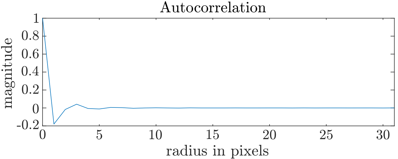
The reason this works is because blue noise textures have correlation only over short distances. At long distances, the values are uncorrelated, as shown in Figure 7.
Figure 7. The autocorrelation of a 64×64 blue noise textures. This shows that pixels that are around seven pixels away from each other can have correlation, while larger distances are uncorrelated.
Ideally if you want N spatiotemporal blue noise values, you should read the blue noise texture at N offsets that are maximally spaced from each other. A good way to do this is to have a progressive low-discrepancy sequence into which you plug the random number index, and it gives you an offset at which to read the texture.
We have had great success using Martin Robert’s R2 sequence to plug in an index, get a 2D vector out in [0,1), and multiply by the blue noise texture size to get the offset at which to read.
There is another way to get multiple values per pixel though, by adding a rank 1 lattice to each pixel. When done this way, it’s similar to Cranley-Patterson rotation on the lattice but using blue noise instead of white noise.
For scalar blue noise, we’ve had good results using the golden ratio or square root of two.
For non-unit vec2 blue noise, we’ve had good results using Martin Robert’s R2 sequence.
This method sometimes converges better than spatiotemporal blue noise but has a more erratic error graph, making it less temporally stable, and damages the blue noise frequency spectrum. Figure 8 shows the frequency damage and Figure 8 shows some convergence behavior. For more information about convergence characteristics, see the simple function convergence section later in this post.
Figure 8. The frequency makeup of golden ratio animated blue noise (top) and spatiotemporal blue noise (bottom). Golden ratio animated blue noise has uneven frequency makeup at various frames, which causes the renderings to be less temporally stable than spatiotemporal blue noise.
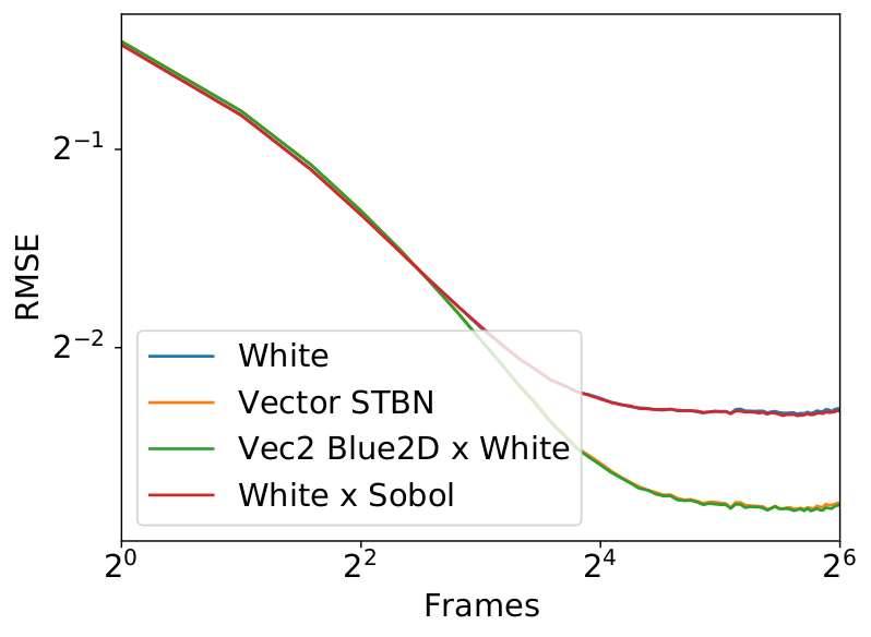
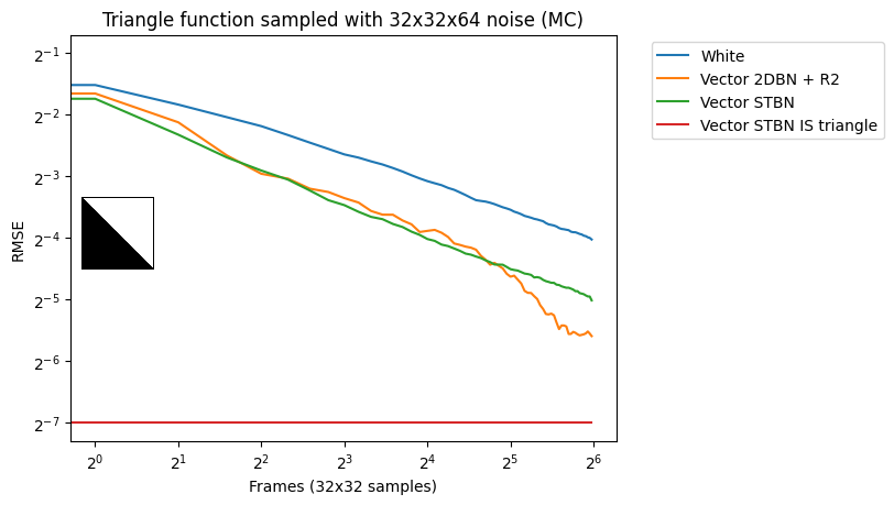
Figure 9 shows a graph comparing real vector spatiotemporal blue noise to the R2 low discrepancy sequence that uses a single vector blue noise texture for Cransley-Patterson rotation.
Figure 9. Convergence rate of various noise types. White noise is worst, and importance sampled spatiotemporal blue noise is best. In the middle, a rank 1 lattice starting with 2D blue noise can do better than uniform spatiotemporal blue noise but is also more erratic and damages the noise spatially.
These two methods are the way that others have animated blue noise previously. Either the blue noise texture is offset each frame, which makes it blue noise over space and white noise over time, or a low-discrepancy sequence is seeded with blue noise values, making it be damaged blue noise over space, but a good converging sequence over time.
Making vector-valued spatiotemporal blue noise through curve inversion
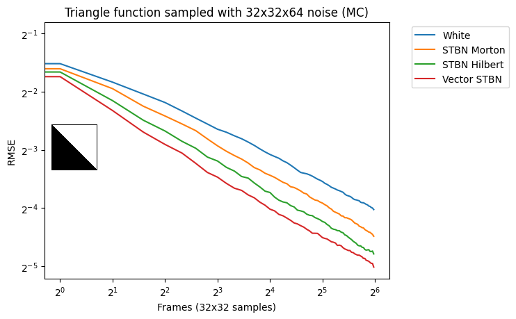
If you have a scalar spatiotemporal blue noise texture, you can put it through an inverted Morton or Hilbert curve to make it into a vector-valued spatiotemporal blue noise texture. We’ve had better results with Hilbert curves. While these textures don’t perform as well as the other methods of making spatiotemporal blue noise, it is much faster and can even be done in real time (Figure 10).
An interesting thing about this method is that we’ve found it works well with all sorts of dither masks or other scalar-valued (grayscale) noise patterns: Bayer matrices, Interleaved Gradient Noise, and even stylized noise patterns.
In all these cases, you get vectors that, when used in rendering, result in error patterns that take the properties and looks of the source texture. This can be fun for stylized noise rendering, but also means that in the future, if other scalar sampling masks are discovered, this method can likely be used to turn them into vector-valued masks with the same properties.
Figure 10. Curve inversion can make vector valued spatiotemporal blue noise, which performs better than white noise, but not as well as vector valued blue noise made with the modified BNDS algorithm.
Stratification
The energy function of vector valued spatiotemporal blue noise can be modified to return nonzero only if the following conditions are true:
The pixels are from the same slice (same z value)
The temporal histograms of the pixels involved in the swap don’t get worse
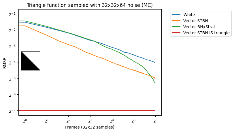
If you do this, you end up with noise that is blue over space but stratified over time; the stratification order is randomized. Because stratification isn’t progressive, it doesn’t converge well until all samples have been taken but does well at that point (Figure 11).
Figure 11. Noise that is blue over space and stratified over time can be made using a modified BNDS algorithm. Convergence graphs show it to be nonprogressive but perform quite well when all samples have been taken.
Higher dimensional blue noise
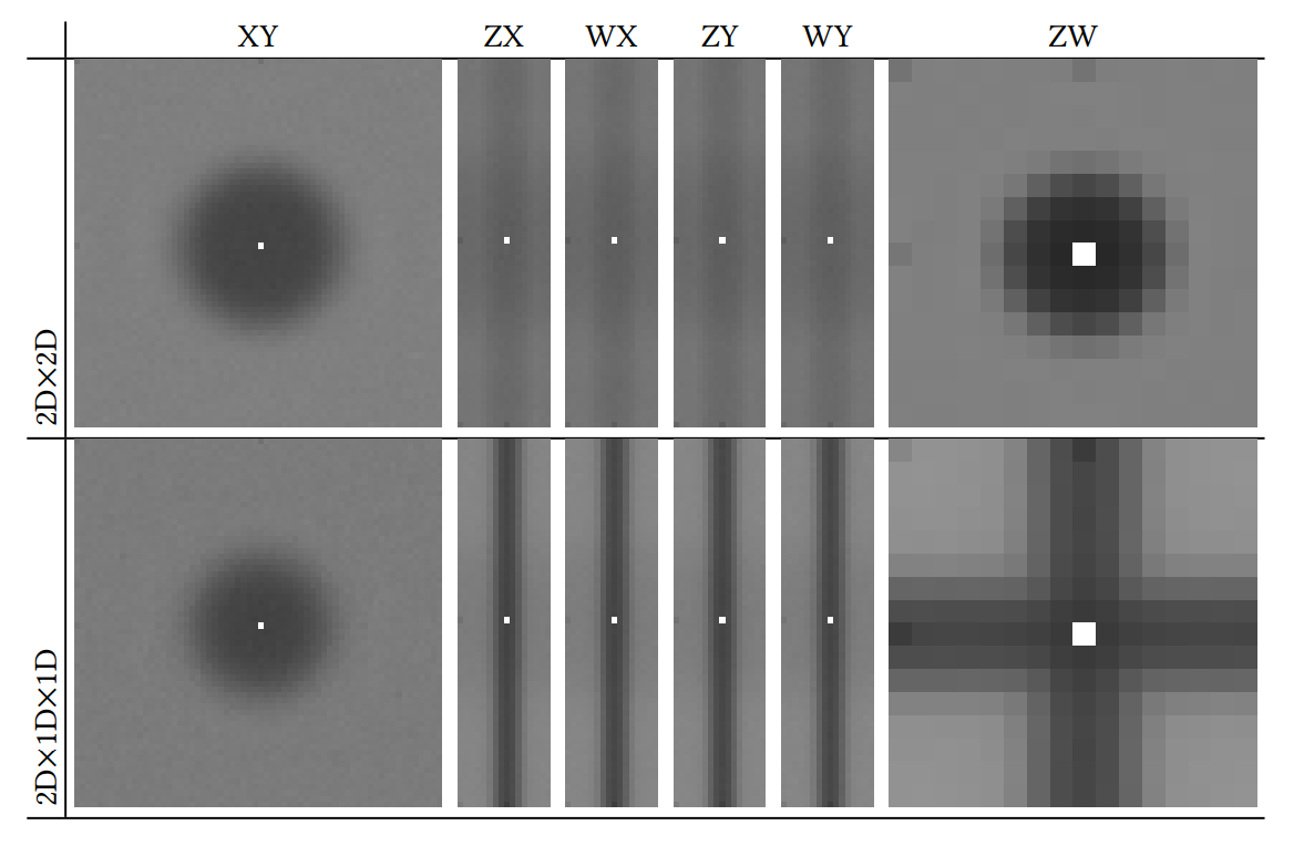
The algorithms for generating spatiotemporal blue noise aren’t limited to working in 3D. The algorithms can be trivially modified to make higher dimensional blue noise of various kinds, although so far, we haven’t been able to find usage cases for them. If spatiotemporal blue noise is 2Dx1D because it is 2D blue noise on XY and 1D blue noise on Z, Figure 12 shows the frequency magnitudes of 4D blue noise, which are 2Dx2D and 2Dx1Dx1D, respectively, with dimensions of 64x64x16x16.
Figure 12. The frequency makeup of 2Dx2D and 2Dx1Dx1D four-dimensional blue noise, on 2D planar projections. The textures are 64x64x16x16.
Point sets
Blue noise textures made with the void and cluster algorithm can be thresholded to a percentage value. That many pixels survive the thresholding and they are blue-noise–distributed. Our scalar-valued spatiotemporal blue noise textures have the same property and result in spatiotemporal blue noise point sets. Figure 13 shows that with the thresholded points of a scalar spatiotemporal blue noise texture, as well as the frequency amplitudes of those thresholded points.
Figure 13. Spatiotemporal blue noise textures thresholded to make spatiotemporal blue noise point sets.
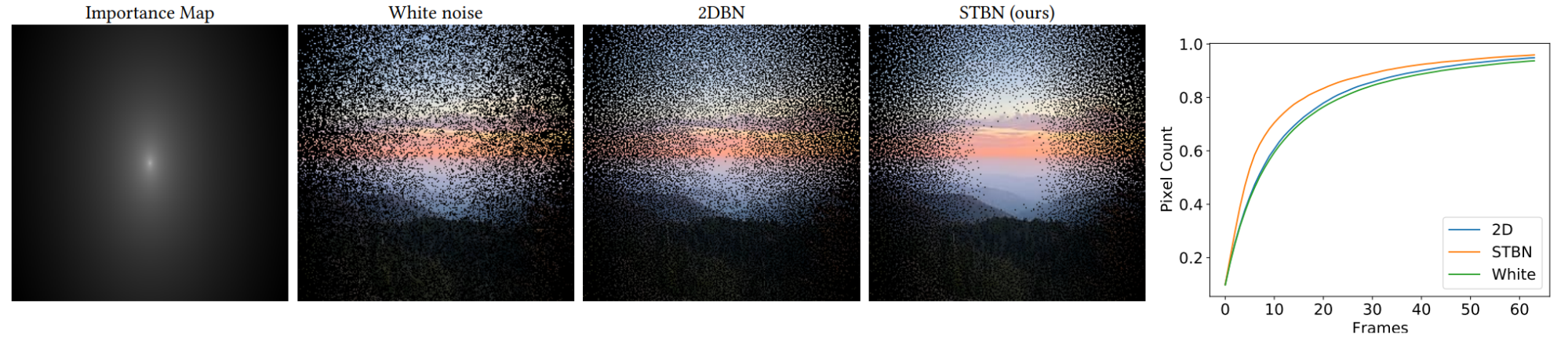
These point sets are such that the pixels each frame are distributed in a pleasing spatial blue noise way, but you also get a different set of points each frame. That means that you get more unique pixels over time compared to white noise or other animated blue noise methods. Figure 14 shows five frames of accumulated samples of an image, using the importance map as the per pixel blue noise threshold value. Our noise samples the most unique pixels the fastest, while also giving a nice blue noise pattern spatially.
Figure 14. Five frames of accumulated samples, using the importance map for stochastic sampling of an image each frame. Spatiotemporal blue noise samples the most unique pixels the fastest, providing the maximum amount of new information each frame.
Simple function convergence
In this section, we discuss the convergence of simple functions using common types of noise, under both Monte Carlo integration and exponential moving average to simulate TAA.
Scalar Monte Carlo integration
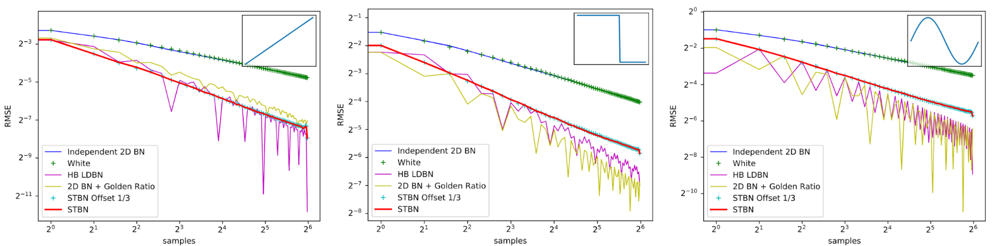
Figure 15 shows convergence rates under Monte Carlo integration, like what you would do when taking multiple samples per pixel. HB LDBN is from A Low-Discrepancy Sampler that Distributes Monte Carlo Errors as a Blue Noise in Screen Space. While low-discrepancy sequences can do better than STBN, it is more temporally stable and also makes perceptually good error by being blue noise spatially. STBN Offset 1/3 shows that if you start STBN from an arbitrary place in the sequence, that it still retains good convergence properties. This shows that STBN is toroidally progressive.
Figure 15. Scalar function convergence using various types of noise under Monte Carlo integration. Spatiotemporal blue noise is not always the best converging, but it does converge significantly better than white noise and is temporally stable.
Scalar exponential moving average
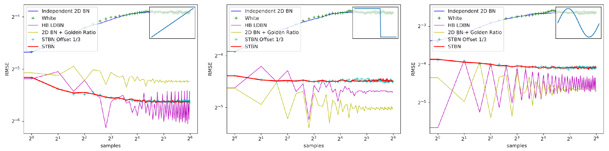
Figure 16 shows convergence rates under exponential moving average. Exponential moving average linearly interpolates from the previous value to the next by a value of 0.1. This simulates TAA without reprojection or neighborhood sampling rejection.
Figure 16. Scalar function convergence using various types of noise under exponential moving average to simulate TAA. Spatiotemporal blue noise is not always the best converging, but it does converge significantly better than white noise and is temporally stable, while also being toroidally progressive as shown by the blue pluses nearly matching the red line.
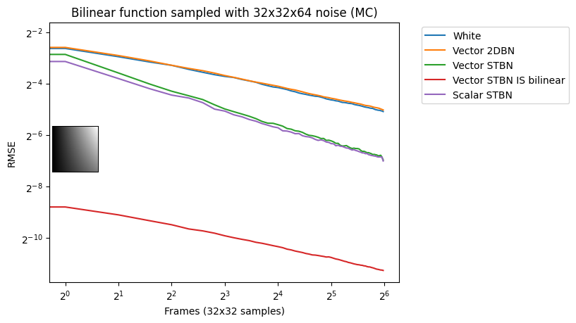
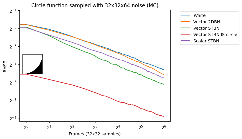
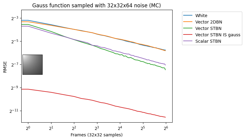
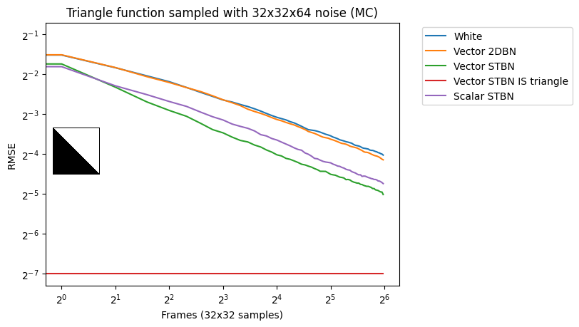
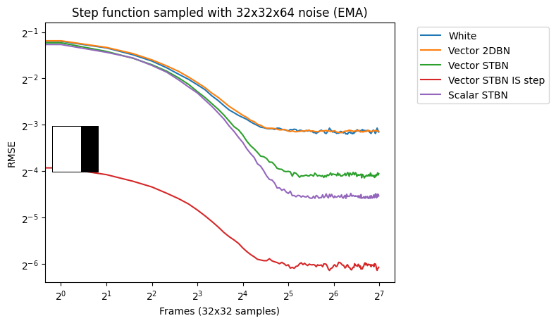
Vec2 Monte Carlo integration
Figure 17 shows convergence rates under Monte Carlo integration. Scalar STBN uses the R2 texture offset method to read two scalar values for this 2D integration. Because of that, it outperforms Vector STBN in the step function, which is ultimately a 1D problem, and also in bilinear, which is ultimately an axis-aligned problem. The reason why importance sampling has any error at all is due to discretization of both the vectors and the PDF values.
Figure 17. Monte Carlo convergence rates of vec2 functions using vec2 noise
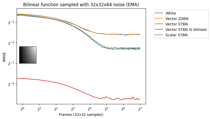
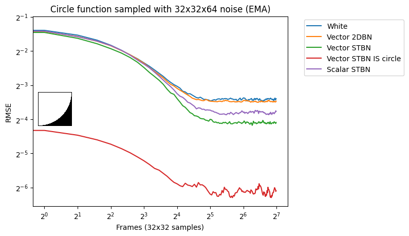
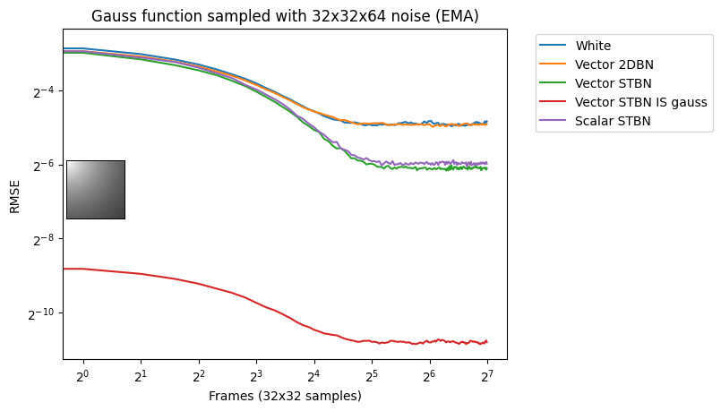
Vec2 exponential moving average
Figure 18 shows convergence under EMA. Exponential moving average linearly interpolates from the previous value to the next by a value of 0.1. This simulates TAA without reprojection or neighborhood sampling rejection.
Figure 18. Exponential moving average convergence rates of vec2 functions using vec2 noise. This simulates behavior under TAA
Conclusion
While blue noise sample points have seen advancements in recent years, blue noise textures seem to have been largely ignored for decades. As shown here, spatiotemporal blue noise textures have several desirable properties for real-time rendering where only low sample counts can be afforded: good spatial error patterns, better temporal stability, and convergence, and toroidal progressiveness, just to name a few.
We believe that these textures are just the beginning, as several other possibilities exist for improvements to sampling textures, whether they are blue-noise–based, hybrids, or something else entirely.
It is worth noting that there are other ways to get great results at the lowest of sample counts, though. For instance, NVIDIA RTXDI is meant for this situation as well but uses a different approach.
Blue noise textures are used in a variety of real time–rendering techniques to hide noise in a perceptually pleasing way
Blue noise textures are useful for providing per-pixel random values to make noise patterns in renderings. Blue noise textures are harder to see and easier to remove than noise made by either random number generators or hashes, both being white noise. To use a blue noise texture, you tile it across the screen, read the texture with nearest neighbor point sampling, and use that as your random value.
In this post, we add the time axis to blue-noise textures, giving each frame high-quality spatial blue noise and making each pixel be blue over time. This provides better convergence and temporal stability over other blue-noise animation methods. We also show you how to make non-uniform blue noise textures to allow for importance sampling. We go on a deeper technical dive in the follow up post, Rendering in Real Time with Spatiotemporal Blue Noise Textures, Part 2.
While othermethods combine blue noise and better convergence, they focus on convergence first and blue noise second. Our work focuses on blue noise first and convergence second, which makes for better renders at the lowest of sample counts, where blue noise has the most benefit.
A notable limitation to blue noise textures is that they work best in low-sample-count, low-dimension algorithms. For high sample counts, or high dimensions found in algorithms like path tracing, you would likely want to switch to low-discrepancy sequences to remove the error, instead of trying to hide it with blue noise.
Also worth mentioning is that that pixels under motion under TAA lose temporal benefits and our noise then functions as purely spatial blue noise. Pixels that are still even for a moment gain temporal stability and lower error, however, which is then carried around by TAA when they are in motion again. In these situations, our noise does no worse than spatial blue noise, so it should always be used instead, to gain benefits where available and do no worse otherwise.
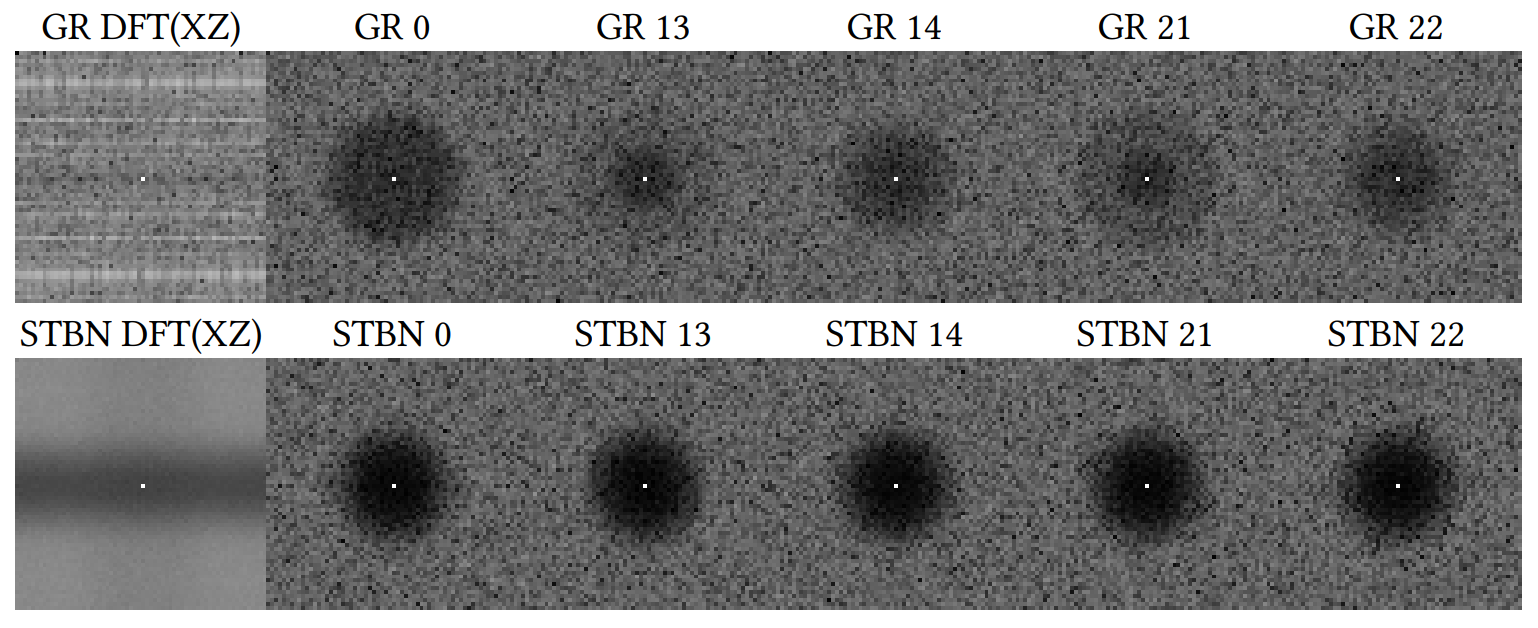
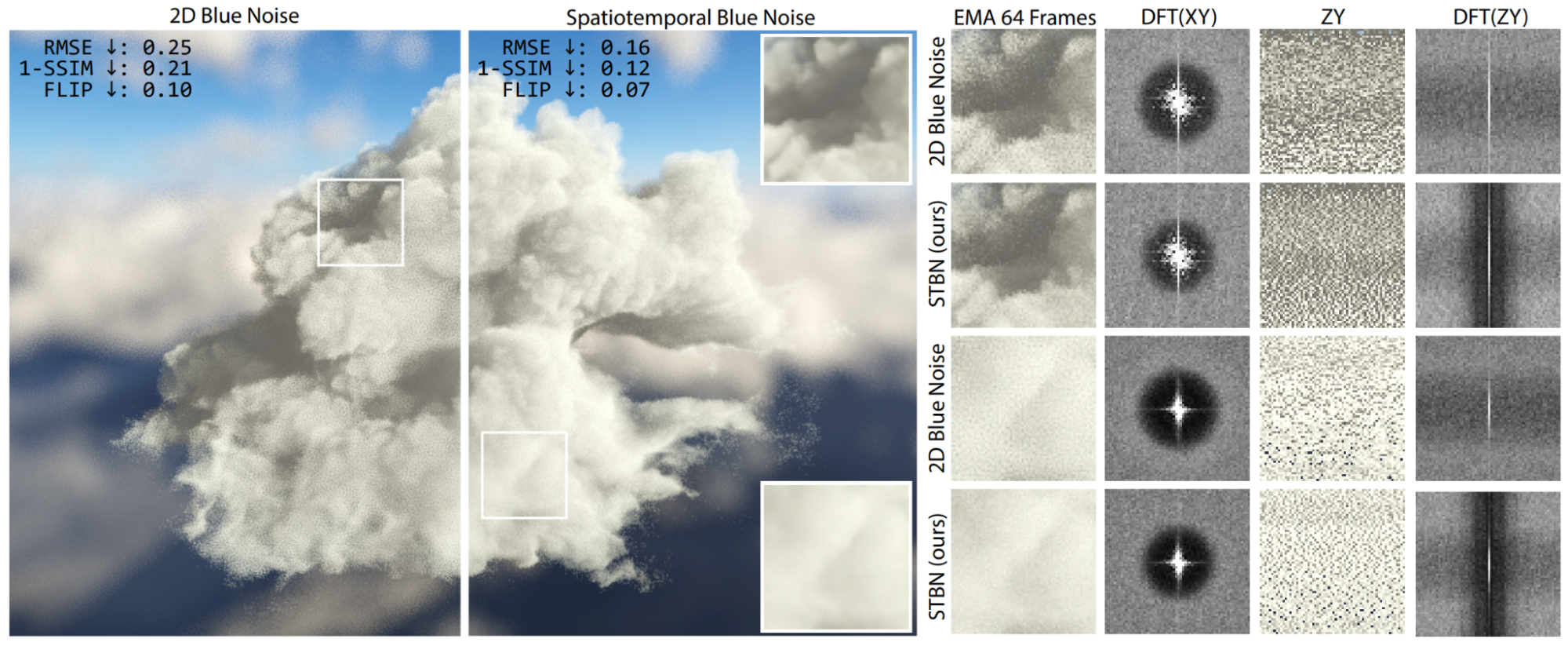
Figure 1 shows an example of using blue noise compared to spatiotemporal blue noise.
Figure 1. The Disney cloud rendered using exponential moving average (EMA) with = 0.1
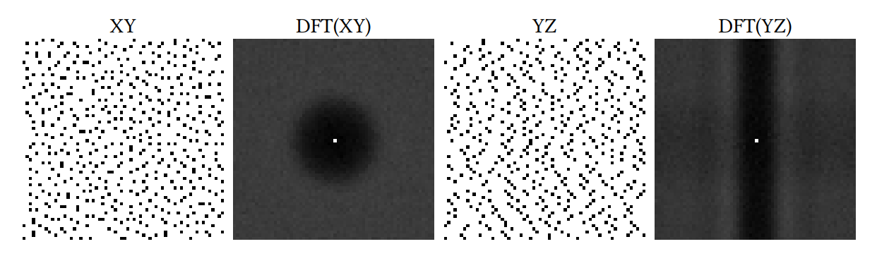
Figure 1 uses stochastic single scattering, where free-flight distances are sampled using a series of blue noise masks over time. Traditional 2D blue noise masks (far left) are easy to filter spatially, but exhibit a white noise signal over time, making the underlying signal difficult to filter temporally.
Our spatiotemporal blue noise (STBN) masks (right of large image) additionally exhibit blue noise in the temporal dimension, resulting in a signal that is easier to filter over time. On the far right, we show two crops of the main image, as well as their corresponding discrete Fourier transforms over both space (DFT(XY)) and time (DFT(ZY)). The Z axis is time. The ground truth is shown in the insets in the large image (upper and lower right corners).
Scalars
Scalar spatiotemporal blue noise textures store a scalar value per pixel and are useful for rendering algorithms that want a random scalar value per pixel, such as stochastic transparency. You generate these textures by running the void and cluster algorithm in 3D but modify the energy function.
When calculating the energy between two pixels, you only return the energy value if the two pixels are from the same texture slice (have the same z value) or if they are the same pixel at different points in time (have the same xy value); otherwise, it returns zero. The result is N textures, which are perfectly blue over space, but each pixel individually is also blue over the z axis (time). In these textures, the (x,y) planes are spatial dimensions that correspond to screen pixels, and the z axis is the dimension of time. You advance one step down the z dimension each frame.
Figure 2 shows example textures and the XY and XZ DFTs for the spatiotemporal blue noise, an array of independent 2D blue noise textures, and 3D blue noise. Only our noise is blue over space (XY) and blue over time (Z), as you can see by the darkening of the center, where the low frequencies are attenuated.
In Figure 2, individual slices of 3D blue noise are not good over space, nor over time. Only our spatiotemporal blue noise is blue over both space and time. For more information about why 3D blue noise is not useful for animating blue noise, see Christoph Peters’ nice explanation in The problem with 3D blue noise.
Figure 2. 2D blue noise is blue over space but not good sampling over time
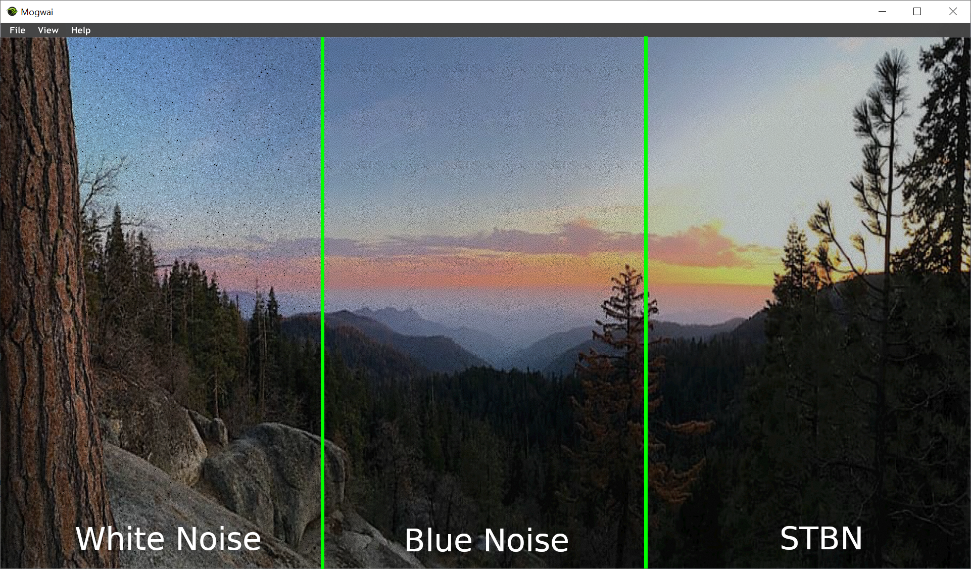
Figure 3 shows a texture that is 50% transparent over a black background, using noise to do a binary alpha test (stochastic transparency) and filtered with temporal anti-aliasing (TAA).
Independent blue noise textures are a significant improvement over white noise by having an evenly spaced set of surviving pixels each frame. This is better for neighborhood sampling rejection, compared to white noise, which has clumps and voids of surviving pixels. Spatiotemporal blue noise does even better by making each pixel survive on frames that are evenly spaced temporally as well, making for a more converged, and more temporally stable result.
Figure 3. Stochastic transparency test of 50% transparency using various types of noise, under TAA
In Figure 3, white noise (left) is very noisy due to clumps and voids that aren’t present in blue noise (center). Our spatiotemporal blue noise does better by having pixels survive evenly not just over space but also over time.
Vectors
Vector spatiotemporal blue noise textures store a vector value per pixel and are useful for rendering algorithms that want a random vector per pixel, such as ray traced ambient occlusion. You generate these textures by running the algorithm from Blue-noise Dithered Sampling (BNDS) in 3D. You make the same modification to the energy function in that paper as you did for scalars in void and cluster. You only return a nonzero energy if they are from the same texture slice, or if they are the same pixel at different points in time.
The result is again N textures, which are perfectly blue over space, but each pixel individually is also blue over the z axis. Unit vectors can be used, which are useful for situations where you need direction vectors, and nonunit vectors can be used, which are useful when you just need an N dimensional random number, such as a point in space.
Figure 4 shows slices of vector valued spatiotemporal blue noise, as well as their frequency components over the space and time axis. This shows that they are blue over space and blue over time.
Vec1
Unit Vec1
Vec2
Unit Vec2
Vec3
Unit Vec3
XY[0]
DFT(XY)
DFT(XZ)
Figure 4. 128x128x64 Spatiotemporal blue noise textures and their frequencies shown for unit and nonunit vectors of dimension 1, 2, and 3.
Figure 5 shows 4 sample per pixel ray traced ambient occlusion (AO) using various types of unit vec3 noise. If a vector is facing towards the normal, it is negated. The difference in quality is apparent between white noise, independent blue noise textures, and spatiotemporal blue noise.
Figure 5. Four-sample per pixel AO using uniformly distributed rays. Blue noise is much better than white noise, and spatiotemporal blue noise is much better than blue noise due to being better sampling over time.
Importance sampling
The BNDS algorithm starts with a set of white noise textures and repeatedly swaps pixels at random, if the swap improves the energy function. There is no reason why these textures must be initialized to uniform white noise vectors, though.
When initializing them to a non-uniform distribution, the algorithm still works in creating blue noise textures. The result is spatiotemporal blue noise textures, which also happen to have a non-uniform histogram, which allows importance sampling. As you need the PDF per pixel to do importance sampling, you can either store the PDF(x) in the alpha channel or calculate the PDF from the value in the texture, such as by doing a dot product if it is cosine hemisphere-weighted or dividing by a normalization value passed in as a shader constant.
Figure 6 shows importance sampled, vector-valued, spatiotemporal blue noise textures.
Texture[0]
DFT(XY)
DFT(ZY)
Importance Map
Cosine Weighted Hemisphere Unit Vec3
N/A
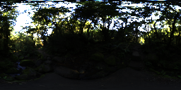
HDR Skybox Importance Sampled Unit Vec3
Figure 6. Slices of importance sampled spatiotemporal blue noise, their DFTs, and the source image they are importance sampling. The alpha channel of the textures stores the PDF as a percentage between the minimum and maximum PDF.
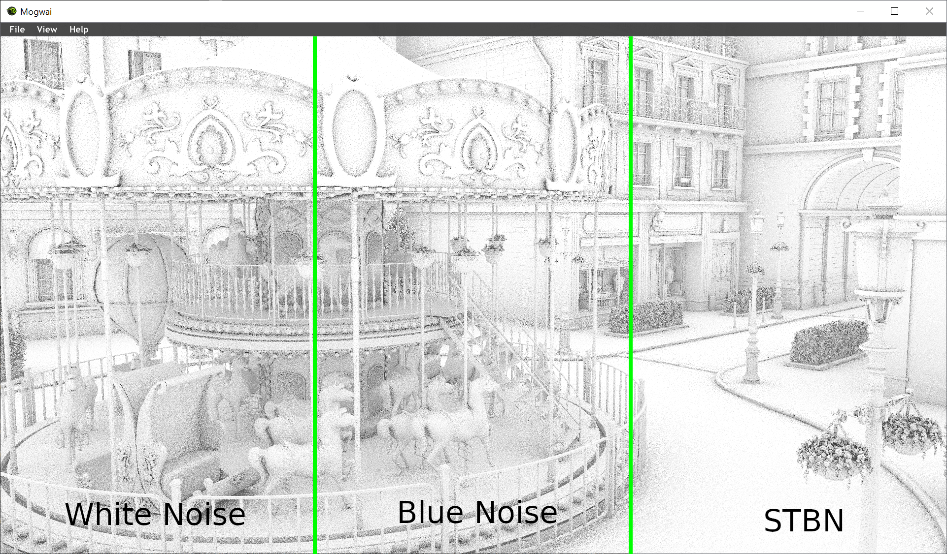
Figure 7 shows four-sample per pixel ray traced AO again but using cosine-weighted–hemisphere, importance-sampled unit vectors. White noise makes a unit vec3, adds it to the normal, and normalizes. Blue noise and STBN have cosine-weighted hemispherical vectors stored in their textures, which are transformed into tangent space using a TBN basis matrix.
Looking at the ovals at the top of the carousel shows how blue noise does better than white noise.
Looking at the window frames in the upper right, you can see how STBN has less noise in the shadows than independent blue noise textures do.
Figure 7. Cosine-weighted hemispherical (importance-sampled) four-sample per pixel ambient occlusion.
In Figure 7, the difference between the noise is less obvious than when uniform sampling but is still there. The noise in blue noise is harder to see and easier to filter than white noise. The noise in STBN is the same way but is also lower magnitude.
Conclusion
Blue noise can be a great way to get better-looking images at low sample counts, like those found in real-time rendering. Blue noise can be useful in nearly any situation that needs one or more random values per pixel.
Have ideas for using blue noise? Download the textures, give it a try, and share your results in the comments. We’d love to see them!
NVIDIA partnered with GeoComputing Group and Lenovo on a high-performance, secure, hybrid platform that enhances productivity for geoscientists.
Whether working remotely or in the office, geoscientists depend on fast access to large and complex datasets to be productive. Yet, up to 40 percent of their time is spent waiting for data to load, with additional time wasted waiting for geoscience applications using high-cost, legacy IT systems.
To improve productivity for geoscientists, GeoComputing Group, Lenovo, and NVIDIA partnered to create a Remote Interpretation and Visualization Appliance (RiVA). The high-performance computing platform was specifically created for subsurface workflows including seismic analysis and reservoir simulation.
Using RiVA, oil and gas enterprises are able to access their data between 50x to 100x faster and reduce model deployment times significantly.
RiVA provides a high-performance, low-latency, consolidated environment for remotely hosted, industry-standard applications used in exploration and production. The platform integrates Lenovo servers and storage with NVIDIA RTX, GPUs, NVIDIA RTX virtual workstations, and Infiniband high-speed networking.
It enables deployment of high-quality, 3D virtual workstations for large datasets and graphically intensive workflows in the oil and gas industry. A Remote Visualization Server (RVS) Module manages the hardware, software, and services for a comprehensive and performant scaling of virtual desktops for petro-technical workflows.
Geoscientists using RiVA can access datasets in a secure data center with a centralized compute model. Applications and data are secured in a private cloud, which helps increase application reliability, speed, and stability. Hybrid workers can overcome productivity drains caused by slow data delivery, delayed application responsiveness, or unexpected downtime.
Oil and gas companies using RiVA have reduced time to production for their infrastructure by up to 70 percent compared to traditional infrastructure builds. They have also experienced between a 100 and 400 percent return on investment in less than a year, providing a more efficient work experience for their geoscientists. With higher accuracy in subsurface analysis and accelerated workflows, enterprises are empowering geoscientists to find more oil in less time.
Explore NVIDIA energy solutions creating a more sustainable future. Learn more about the RiVA high-performance computing platform in the video below.
Figure 1. A day in the life of a GeoScientist introduces RiVA from GeoComputing, Lenovo, and NVIDIA.
2021 saw massive growth in the demand for edge computing — driven by the pandemic, the need for more efficient business processes, as well as key advances in the Internet of Things, 5G and AI. In a study published by IBM in May, for example, 94 percent of surveyed executives said their organizations will implement Read article >
I want to generate time series tabular data. Most of generative deep learning models consists of VAE and/or GAN which are for most part relating to images, videos, etc.
Can you please point me to relevant tutorial souces (if it includes code along with theory, all the more better) pertaining to synthethic time series data generation using deep learning models or other techniques?
Hey guys, I know this may not be the perfect place, but I though some of you may have the skills and the interest to apply to some recent job openings. I you are not interested in these jobs just ignore them, downvote them, but there may be other who not only find them useful but they can make a difference if you are interested in them apply directly to the link, we are searching for North America based individuals (for tax reasons)only, thanks!
This post covers the validation of camera models in DRIVE Sim, assessing the performance elements, from rendering of the world scene to protocol simulation.
Autonomous vehicles require large-scale development and testing in a wide range of scenarios before they can be deployed.
Simulation can address these challenges by delivering scalable, repeatable environments for autonomous vehicles to encounter the rare and dangerous scenarios necessary for training, testing, and validation.
NVIDIA DRIVE Sim on Omniverse is a simulation platform purpose-built for development and testing of autonomous vehicles (AV). It provides a high-fidelity digital twin of the vehicle, the 3D environment, and the sensors needed for the development and validation of AV systems.
Unlike virtual worlds for other applications such as video games, DRIVE Sim must generate data that accurately models the real-world. Using simulation in an engineering toolchain requires a clear grasp of the simulator’s performance and limitations.
This accuracy covers all of the functions modeled by the simulator including vehicle dynamics, vehicle components, behavior of other drivers and pedestrians, and the vehicle’s sensors. This post covers part of the validation of camera models in DRIVE Sim, which requires assessing the individual performance of each element, from rendering of the world scene to protocol simulation.
Validating a camera simulation model
A thorough validation of a simulated camera can be performed with two methodologies:
Individual analysis of each component of the model ( Figure 1).
A top-down verification that the camera data produced by a simulator accurately represents the real camera data in practice, for instance, by comparing the performance of perception models trained on real or synthetic images.
Individual component analysis is a complex topic. This post describes our component-level validation of two critical properties of the camera model: camera calibration (extrinsic and intrinsic parameters) and color accuracy. Direct comparisons are made with real world camera data to identify any delta between simulated and real world images.
Figure 1. Summary of camera model components
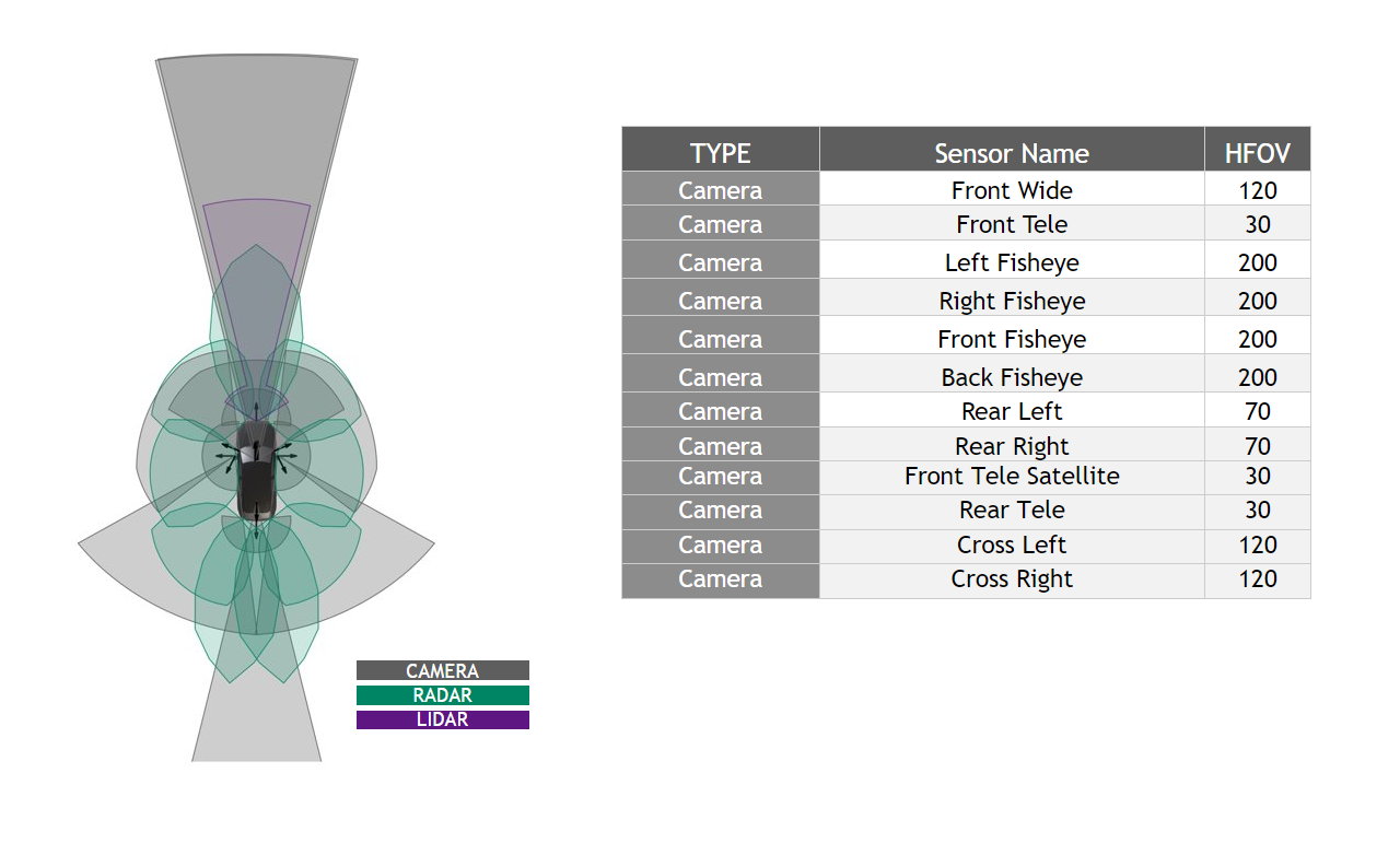
For this validation, we chose to use a set of camera models from the NVIDIA DRIVE Hyperion sensor suite. Figure 2 details the camera models used throughout testing.
Figure 2. NVIDIA DRIVE Hyperion 8 sensor set
Camera calibration
AV perception requires a precise understanding of where the cameras are positioned on the vehicle and how each unique lens geometry of a camera affects the images it produces. The AV system processes these parameters through camera calibration.
A simulated camera sensor should accurately reproduce the images of a real camera when subjected to the same calibration and a digital twin environment. Likewise, simulated camera images should be able to produce similar calibration parameters as their real counterparts when fed into a calibration tool.
We use NVIDIA Driveworks, our sensor calibration interface, to estimate all camera parameters mentioned in this post.
Validation of camera characteristics can be done in these steps:
Extrinsic validation: Camera extrinsics are the characteristics of a camera sensor that describe its position and orientation on the vehicle. The purpose of extrinsic validation is to ensure that the simulator can accurately reproduce an image from a real sensor at a given position and orientation.
Calibration validation: The accuracy of the calibration is verified by computing the reprojection error. In real-world calibrations, this approach is used to quantify whether the calibration was valid and successful. We apply this step here to calculate the distance between key detected features reprojected on real and simulated images.
Intrinsic validation
Intrinsic camera calibration describes the unique geometry of an individual lens more precisely than its manufacturing tolerance by setting coefficients of a polynomial.
is the distance in pixels to the distortion center
are the coefficients of the distortion function
(theta) is the resulting projection angle in radians
The calibration of this polynomial enables an AV to make better inferences from camera data by characterizing the effects of lens distortion. The difference between two lens models can be quantified by calculating the max theta distortion between them.
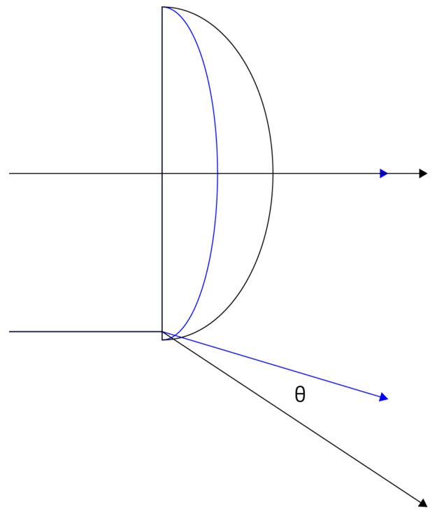
Figure 3. Max theta distortion diagram
Max theta distortion describes the angular difference of light passing through the edge of a lens (corresponding to the edge of an image), where distortion is maximized. In this test, we will use the max theta distortion to describe the difference between a lens model generated from real calibration images and one from synthetic images.
We validate the intrinsic calibration of our simulated cameras according to the following process:
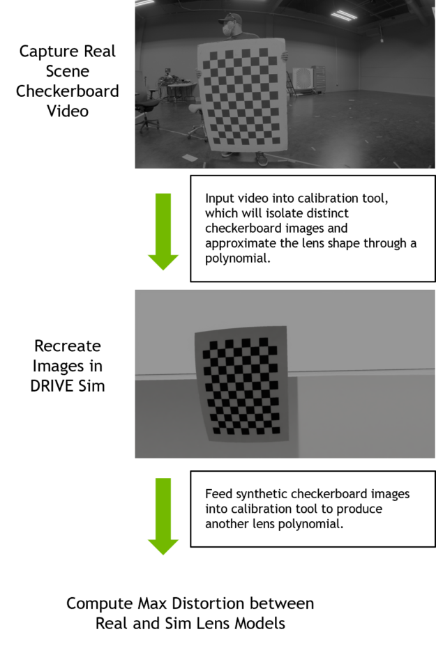
Figure 4. Intrinsic validation process
Perform intrinsic camera calibration: Mounted cameras on a vehicle or test stand capture video of a checkerboard chart moving through each camera’s field of view at varying distances and degrees of tilt. This video is input into the DriveWorks Intrinsics Constraints Tool, which will pull distinct checkerboard images from it and output the polynomial coefficients for each camera in the calibration.
Produce simulated checkerboard calibration images: The real camera lens calibration data are used to recreate each camera in DRIVE Sim. We recreate the real checkerboard images in simulation from the estimated chart positions and orientations output by the calibration tools.
Produce intrinsic calibration from synthetic images: We input synthetic images into DriveWorks calibration tools to produce new polynomial coefficients.
Compute max theta distortion from real to simulated lens: For each lens, we compare the geometry defined by the calibration from real images to the geometry defined by the calibration from the simulated images. We then find the point where the angle that light passes through varies most between the two lenses. The variation is reported as a percentage of the theoretical field of view of that lens (/(FOV*100)).
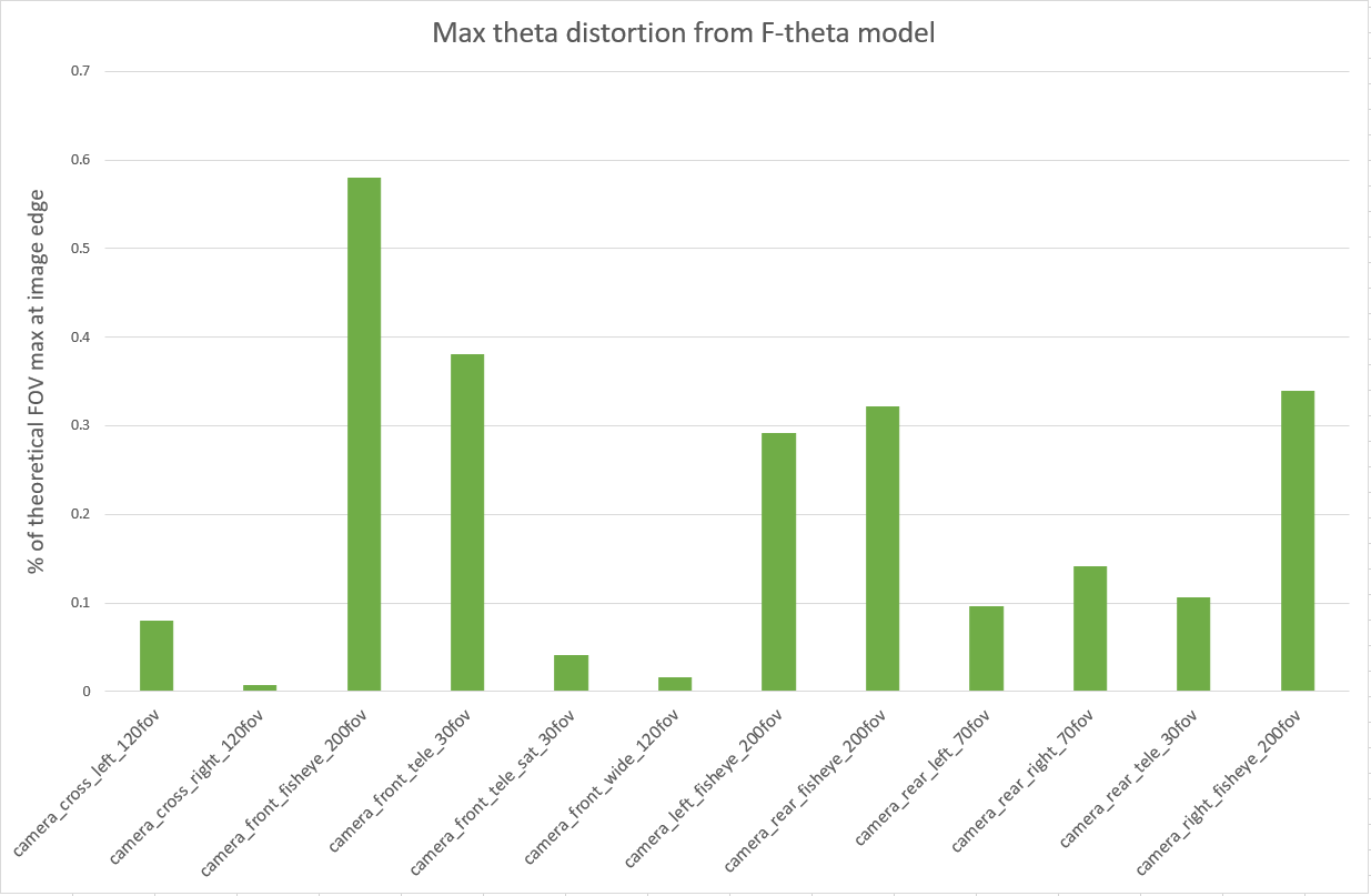
The max theta distortion for each camera derived by comparing its real f-theta lens calibration to the calibration yielded from simulated images.
Figure 5. Max theta distortion from F-theta model
This first result exceeded our expectations as the simulation is behaving predictably and reproducing the observed outcomes from real-world calibrations.
This comparison provides a first degree of confidence in the ability of our model to accurately represent lens distortion effects because we observe a small discrepancy between real and simulated cameras. The front telephoto lens is difficult to constrain in real life, hence we expected it to be an outlier in our simulation results.
The fisheye cameras calibrations exhibit the largest real-to-sim difference (0.58% of FOV for the front fisheye camera).
Another way to look at these results is by considering the effect of the distortions on the generated images. We compare the real and simulated detected features from the calibration charts in a later step, described under the Numerical Feature Marker comparison.
We proceed with the extrinsic validation method.
Extrinsic validation
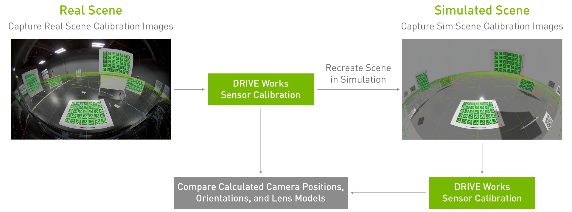
We validate the extrinsic calibration of our simulated cameras according to the following process:
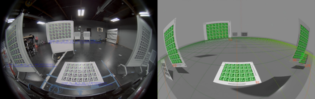
Perform extrinsic camera calibration: Mounted cameras on a vehicle or test stand capture images of multiple calibration patterns (AprilTag charts) located throughout the lab. For our test, cameras were mounted per the NVIDIA DRIVE Hyperion Level 2+ reference architecture. Using the DriveWorks calibration tool, we calculate the exact position and orientation of the camera and the calibration charts in 3D space.
Recreate scene in simulation: Using extrinsic parameters from real calibration and ground truth of AprilTag chart locations, the cameras and charts are spawned in simulation at the same relative positions and orientations as in the real lab. The system generates synthetic images from each of the simulated cameras.
Produce extrinsic calibration from synthetic images and compare to real calibration: Synthetic images are inputted into DriveWorks calibration tools to output the position and orientation of all cameras and charts in the scene. We calculate the 3D differences between extrinsic parameters derived from real vs. synthetic calibration images.
Figure 6. Extrinsic validation process
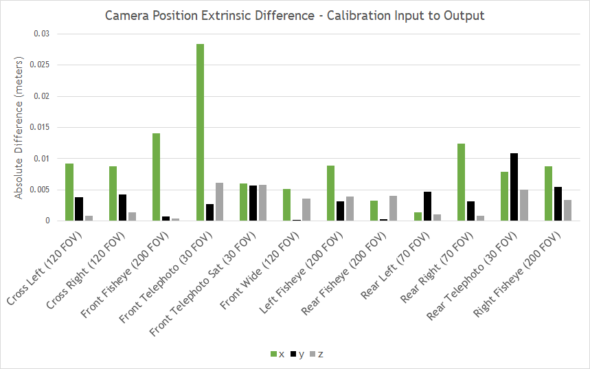
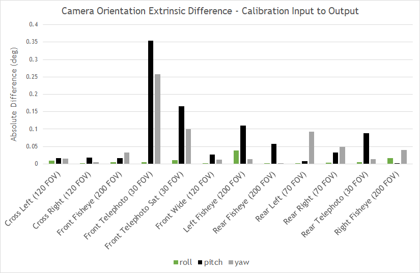
Figure 7 shows the differences in extrinsic parameters for each of the 12 cameras on the tested camera rig, comparing the real camera calibration to the calibration yielded by the simulated camera images. All camera position parameters matched within 3 cm and all camera orientation parameters matched within 0.4 degrees.
All positions and orientations are given with regard to a right-handed reference coordinate system with origin at the center of the rear axle of the car projected onto the ground plane, where x aligns with the direction of the car, y to the left, and z up. Yaw, pitch, and roll are counter-clockwise rotations around z, y, and x.
Figure 7. Camera position extrinsic differences–calibration input to output
Figure 8. Camera orientation extrinsic differences–calibration input to output
Results
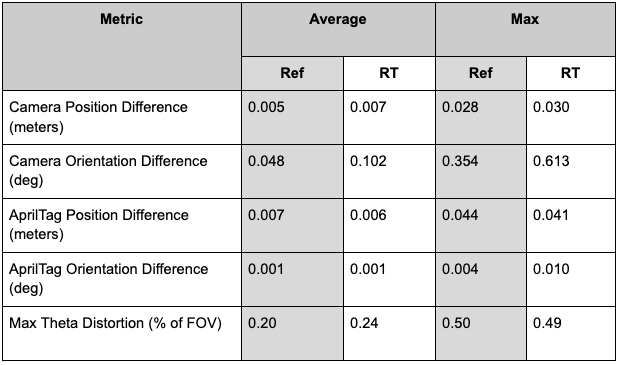
The validation previously described compares real lab calibrations to digital twins’ calibrations in DRIVE Sim RTX renderer. The RTX renderer is a path-tracing renderer that provides two rendering modes, a real-time mode and a reference mode (not real-time, focus on accuracy) to provide full flexibility depending on the specific use case.
This full validation process was done with digital twins rendered in both RTX real-time and reference modes to evaluate the effect of reduced processing power allocated to rendering. See a summary of the real-time validation results in the following table, with reference results available for comparison.
As expected, there was a slight increase in real-to-sim error for most measurements when rendering in real-time due to reduced image quality. Nonetheless, calibration based on real-time images matched lab calibrations within 0.030 meters and 0.041 degrees for cameras, 0.041 meters and 0.010 degrees for AprilTag locations, and 0.49% of theoretical field of view for the lens models.
Figure 9. Reference vs. real-time validation results
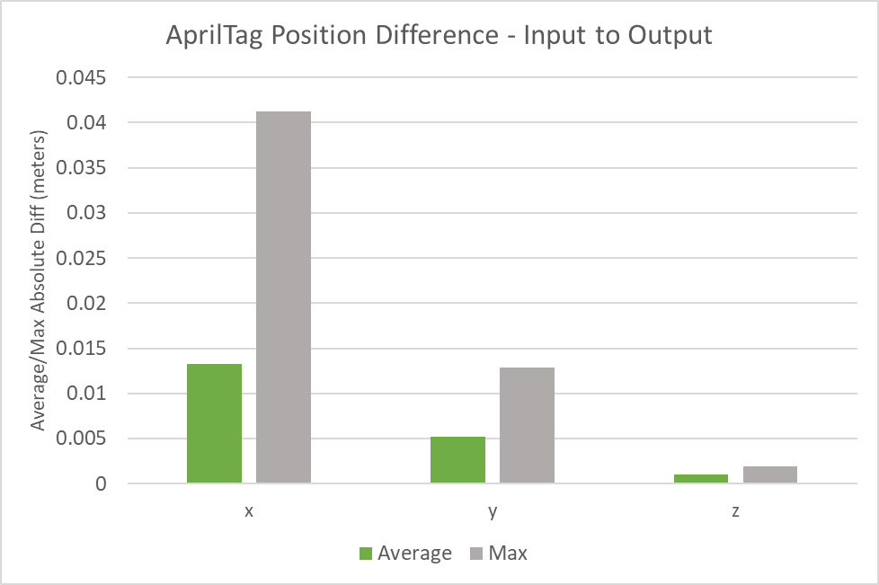
The following figures indicate the average and max position or orientation differences across 22 AprilTag charts located in the real and simulated environments. The average position difference from the real charts to their digital twins was less than 1.5 cm along all axes and no individual chart’s position difference exceeded 4.5 cm along any axis.
The average orientation difference from the real charts to their digital twins was less than 0.001 degrees for all axes and no individual chart’s orientation difference exceeded 0.004 degrees along any axis.
Figure 10. Average/max AprilTag orientation differences–calibration input to output
There is currently no standard to define an acceptable error under which a sensor simulation model can be deemed viable. Thus, we compare our position and orientation delta values to the calibration error yielded by real-world calibrations to define a valid criterion for the maximum acceptable error for our simulation. The resulting errors from our tests are consistently smaller than the calibration error observed in the real world.
This calibration method is based on statistical optimization techniques used by our calibration tool and hence can introduce its own uncertainty. However, it is also important to note that the DriveWorks calibration system has been consistently used in research and development for sensor calibration with a high degree of accuracy.
These results also demonstrate that the calibration tool can function with simulation-rendered images and provide comparable results with the real world. The fact that the real-world calibration system and our simulation are in agreement is a first significant indicator of confidence for our camera simulation model.
Moreover, this method also validates the simulator as a whole, because the digital twin used for calibration models the scene in its entirety with all 12 cameras, without tweaking values to improve results.
To assess further the validity of this method, we then run a direct numerical feature marker comparison between the real and simulated images.
Numerical feature markers comparison
The calibration tool provides a visual validator to reproject the calibration charts positions onto the input images based on the estimated intrinsic parameters. The images show an example of the overlay of the detected features and the reprojection statistics (mean, std, min, and max reprojection error) for the simulated and real camera.
Figure 11. Overlay target positions onto input images for camera_rear_fisheye_200fov
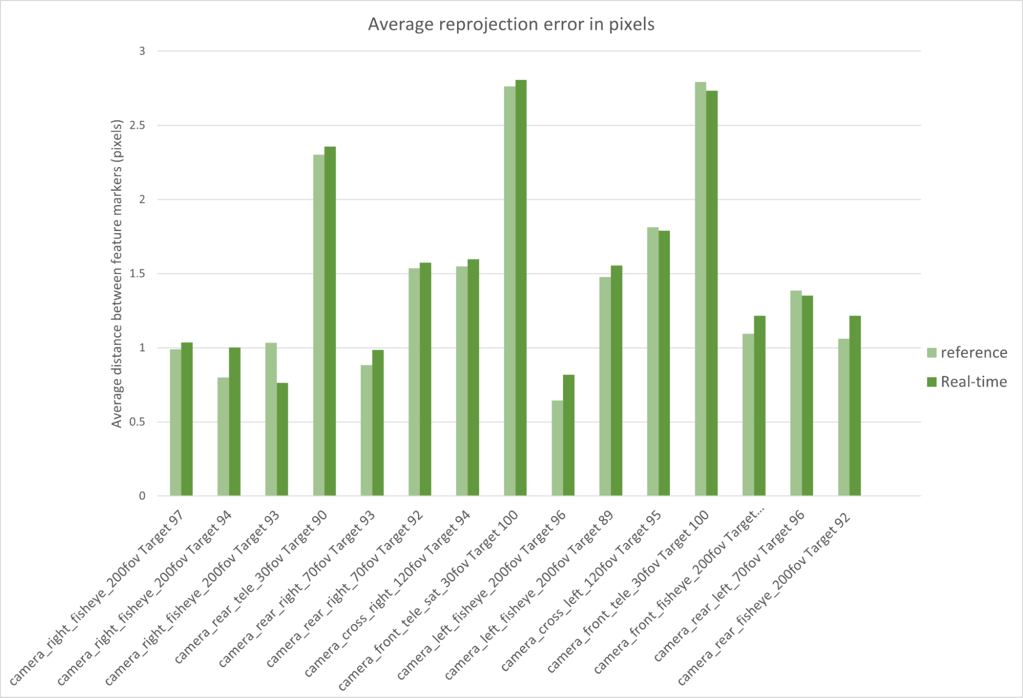
Computing the reprojection error enables us to assert further the validity of the prior calibration method. This approach parses the calibration tool’s detected features and compares them to the ones in the real image.
Here we consider the corners of each of the AprilTags in the calibration charts as the feature markers. We calculate the distance in pixels between the feature markers detected on real images compared to synthetic images, both for path-traced and real-time simulation.
The following figure shows an average distance of 1.4 pixels between reference path-traced simulated and real feature markers. The same comparison based on the real-time simulated dataset yields an average reprojection error of 1.62 pixels.
Figure 12. Average reprojection error (reference vs. real time)
Both values are the real-world projection error threshold of 2 pixels used to evaluate the accuracy of the real-world calibrations. The results are very promising, in particular because this method is less dependent on the inner workings of our calibration tool.
In fact, the calibration tool is only used here to estimate the detected feature markers in each image. The comparison of the markers is done based on a purely algorithmic analysis of objects in 3D space.
Color accuracy assessment
The camera calibration results demonstrate pixel correspondence of images produced by our camera sensor model to their real image counterparts. The next step is to validate that the values associated with each of those pixels are accurate.
We simulated a Macbeth ColorChecker chart and captured an image of it in DRIVE Sim to validate image quality. The RGB values of each color patch were then compared to those of the corresponding real image.
In addition to the real images, we also introduced the Iray renderer, NVIDIA’s most realistic physical light simulator, validated against CIE 171:2006. We performed this test first using simulated images generated with the Iray rendering system, then with NVIDIA RTX renderer. The comparison with Iray gives a good measure of the capability of the RTX renderer against a recognized industry gold standard.
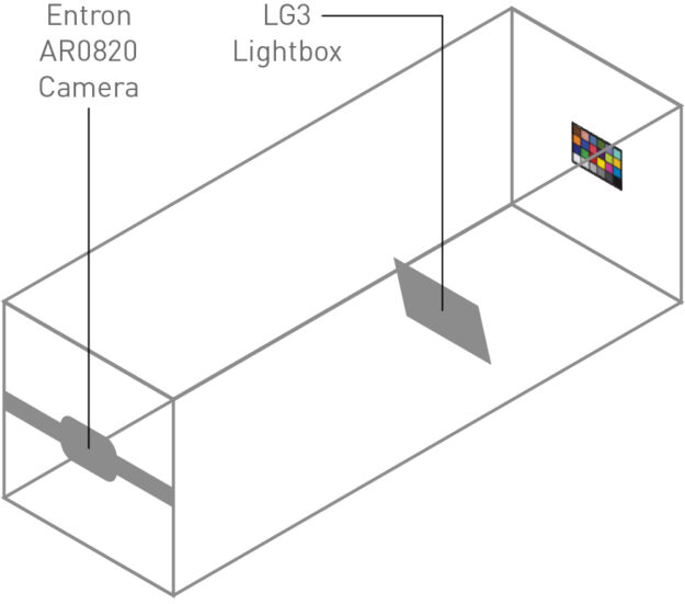
Figure 13. Image quality test setup
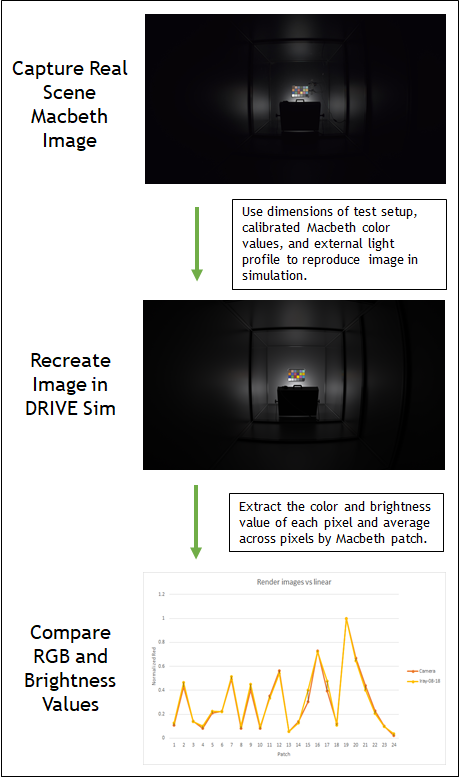
We validate the image quality of our simulated cameras according to the following process:
Capture image of Macbeth ColorChecker chart in test chamber: A Macbeth ColorChecker chart is placed at a measured height and illuminated with a characterized external light source. The camera is placed at a known height and distance from the Macbeth chart.
Re-create image in simulation: Using the dimensions of the test setup, calibrated Macbeth chart values, and the external lighting profile, we render the test scene using the DRIVE Sim RTX renderer. We then use our predefined camera model to recreate the images captured in the lab.
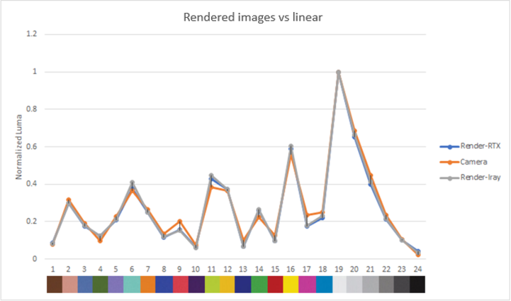
Extract mean brightness and RGB values for each patch: We average the color values across all pixels in each patch for all three images (real, Iray, DRIVE Sim RTX renderer).
Compare white-balanced brightness and RGB values: Measurements are normalized for each patch against patch 19 for white-balancing. We compare the balanced color and brightness values across the real image, Iray rendering, and RTX rendering.
Figure 14. Macbeth ColorChecker test process
Figure 15. Macbeth ColorChecker reference chart
Figure 16. Real and rendered luma and RGB comparisons
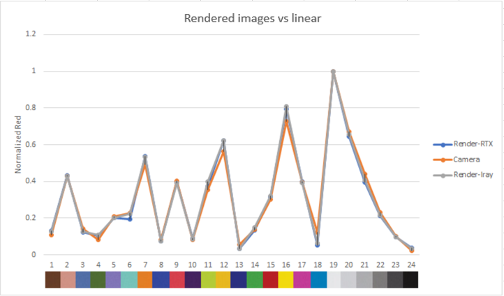
Figure 17. Comparison of red color contributions, rendered images vs real image
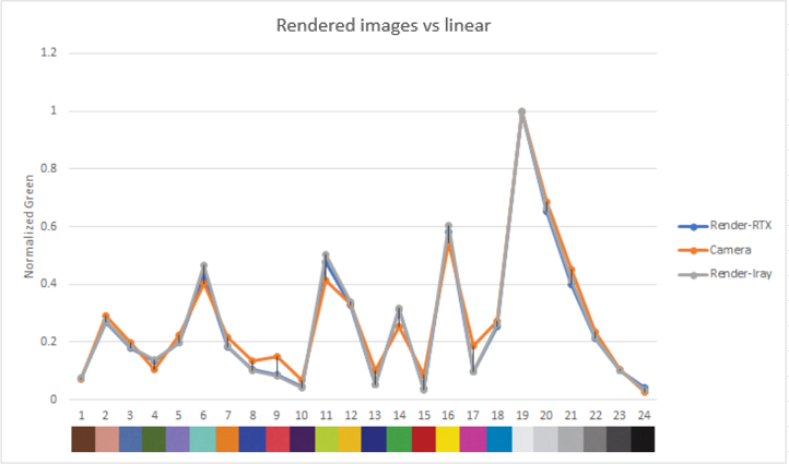
Figure 18. Comparison of green color contributions, rendered images vs real image
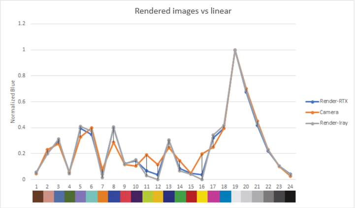
Figure 19. Comparison of blue color contributions, rendered images vs real image
The graphs show the normalized luma and RGB output for each color patch in the rendered and real images.
Both the luma and RGB values for our rendered images are close to the real camera, which gives confidence in the ability of our sensor model to reproduce color and brightness contributions accurately.
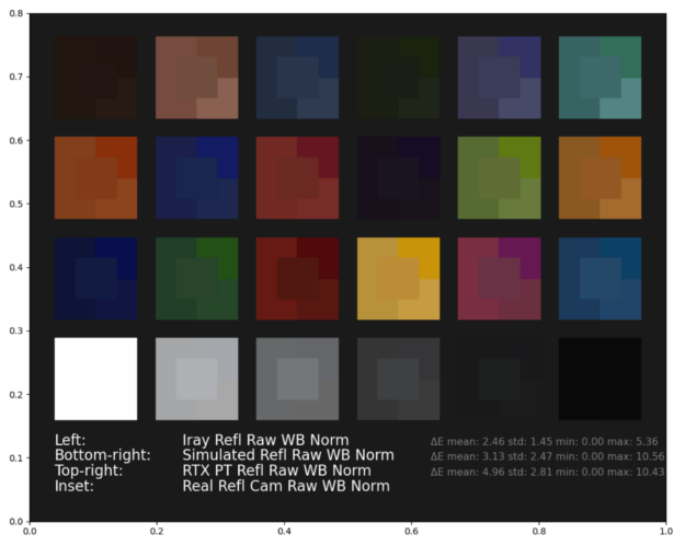
For a direct visual comparison, we show the stitched white-balanced RGB values of the Macbeth chart real and synthetic images (Iray, real-time, and path-traced contributions).
Figure 20. Stitched RGB patches Macbeth color chart (synthetic vs. real)
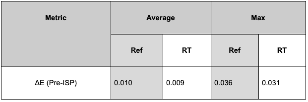
We also compute ΔE (see results in Figure 22), a CIE2000 computer vision metric, which quantifies the distance between the rendered and original camera values and is often used for camera characterization. A lower ΔE value indicates greater color accuracy and the human eye cannot detect a value under 1.
Figure 21. Reference vs. real-time results for CIE2000
While ΔE provides a good measure of perceptual color difference and is recognized as an imaging standard, it is limited to human perception. The impact of such a metric on a neural network will remain to be evaluated in further tests.
Conclusion
This post presented the NVIDIA validation approach and preliminary results for our DRIVE Sim camera sensor model.
We conclude that our model can accurately reproduce real cameras’ calibrations parameters with an overall error that is below real-world calibration error.
We also quantified the color accuracy of our model with reference to the industry standard Macbeth color checker and found that it is closely aligned with typical R&D error margins.
In addition, we conclude that RTX real time rendering is a viable tool to achieve this level of accuracy.
This confirms that the DRIVE Sim camera model can reproduce the previously mentioned parameters of a real-world camera in a simulated environment at least as accurately as a twin camera setup in the real world. More importantly, these tests provide confidence to users that the outputs of the camera models, as far as intrinsics, extrinsics, and color reproduction, will be accurate and can serve as a foundation for other validation work to come.
The next steps will be to validate our model in the context of its real-world perception use cases and provide further results on imaging KPIs for the model in open-loop.
The thing about inspiration is you never know where it might come from, or where it might lead. Anderson Rohr, a 3D generalist and freelance video editor based in southern Brazil, has for more than a dozen years created content ranging from wedding videos to cinematic animation. After seeing another creator animate a sci-fi character’s Read article >
The future of cloud gaming is available NOW, for everyone, with preorders closing and GeForce NOW RTX 3080 memberships moving to instant access. Gamers can sign up for a six-month GeForce NOW RTX 3080 membership and instantly stream the next generation of cloud gaming, starting today. Snag the NVIDIA SHIELD TV or SHIELD TV Pro Read article >

 Spatiotemporal blue noise textures add the time axis, providing better convergence of blue noise, without loss of quality of the blue noise error patterns.
 , small changes in x result in small changes in y, and that big changes in x result in big changes in y.


 = 0.1
= 0.1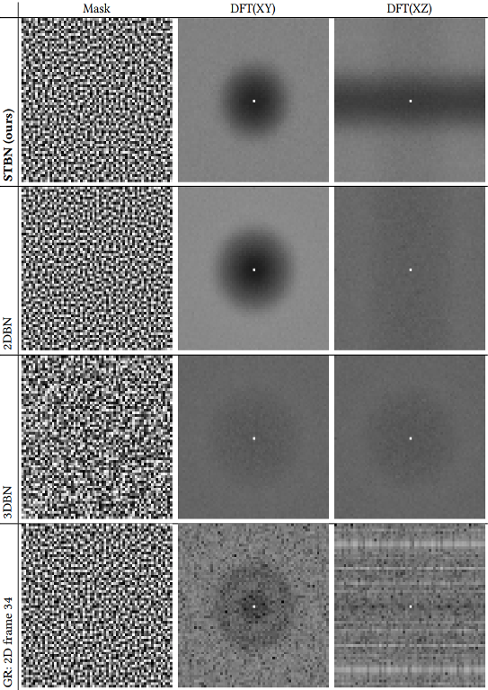


 NVIDIA partnered with GeoComputing Group and Lenovo on a high-performance, secure, hybrid platform that enhances productivity for geoscientists.
 This post covers the validation of camera models in DRIVE Sim, assessing the performance elements, from rendering of the world scene to protocol simulation.
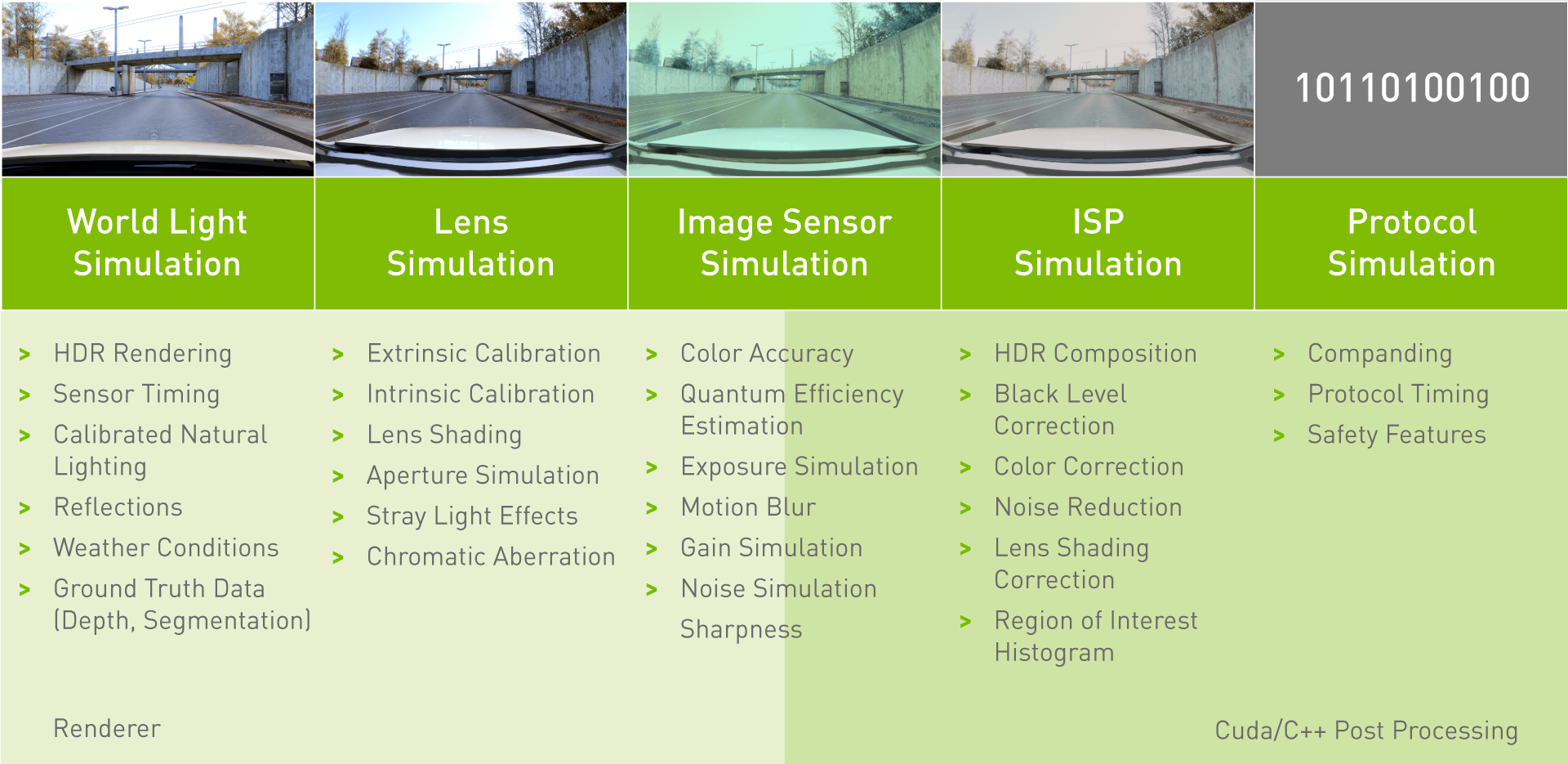

 is the distance in pixels to the distortion center
 are the coefficients of the distortion function
 (theta) is the resulting projection angle in radians