Categories
Misc

Discovering New Features in CUDA 11.4

NVIDIA announces the newest release of the CUDA development environment, CUDA 11.4. This release includes GPU-accelerated libraries, debugging and optimization tools, programming language enhancements, and a runtime library to build and deploy your application on GPUs across the major CPU architectures: x86, Arm, and POWER. CUDA 11.4 is focused on enhancing the programming model and … Continued

NVIDIA announces the newest release of the CUDA development environment, CUDA 11.4. This release includes GPU-accelerated libraries, debugging and optimization tools, programming language enhancements, and a runtime library to build and deploy your application on GPUs across the major CPU architectures: x86, Arm, and POWER.

CUDA 11.4 is focused on enhancing the programming model and performance of your CUDA applications. CUDA continues to push the boundaries of GPU acceleration and lay the foundation for new applications in HPC, graphics, CAE applications, AI and deep learning, automotive, healthcare, and data sciences.

CUDA 11.4 has several important features. This post offers an overview of the key capabilities:

  • CUDA Programming model enhancements:
    • CUDA Graphs
    • Multi-Process Service (MPS)
    • Formalizing Asynchronous Data Movement
  • C++ Language support – CUDA
  • Compiler enhancements
  • CUDA Driver Enhancements

CUDA 11.4 ships with the R470 driver, which is a long-term support branch. GPUDirect RDMA and GPUDirect technology Storage (GDS) are now part of the CUDA Driver and Toolkit. This streamlines the workflow and enables our developers to leverage these technologies without the need for separate installation of additional packages. The driver enables new MIG configurations for the recently launched NVIDIA A30 GPU, which doubles the memory per MIG slice. This results in greater peak performance for various workloads on the A30 GPU, especially for AI inference workloads.

CUDA 11.4 is available to download.

CUDA programming model enhancements

This release introduced key enhancements to improve the performance of CUDA Graphs without requiring any modifications to the application or any other user intervention. It also improves the ease of use of Multi-Process Service (MPS). We formalized the asynchronous programming model in the CUDA Programming Guide.

CUDA Graphs

Reducing graph launch latency is a common request from the developer community, especially in applications that have real-time constraints, such as 5G telecom workloads or AI inference workloads. CUDA 11.4 delivers performance improvements in reducing the CUDA graph launch times. In addition, we also integrated the stream-ordered memory allocation feature that was introduced in CUDA 11.2.

For more information, see CUDA Graphs in the CUDA Toolkit Programming Guide and Getting Started with CUDA Graphs.

Performance improvements

CUDA graphs are ideal for workloads that are executed multiple times, so a key tradeoff in choosing graphs for a workload is amortizing the cost of creating a graph over repeated launches. The higher the number of repetitions or iterations, the larger the performance improvement.

In CUDA 11.4, we made a couple of key changes to CUDA graph internals that further improve the launch performance. CUDA graphs already sidesteps streams to enable lower latency runtime execution. We extended this, to bypass streams even at the launch phase, submitting a graph as a single block of work directly to the hardware. We’ve seen good performance gains from these host improvements, both for single-threaded and multithreaded applications.

Figure 1 shows the relative improvement in launch latency for the re-launch of different graph patterns. There is significant benefit for graphs that have a fork or join pattern.
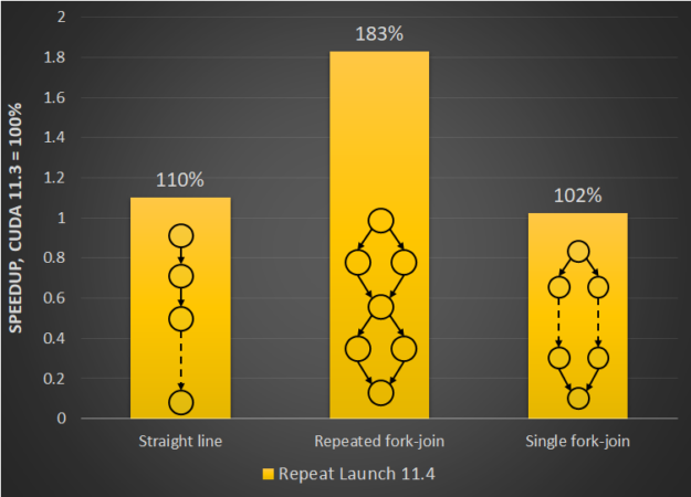
Figure showing the relative launch latency improvements in CUDA 11.4 for repeat launches of a single graph for different graph patterns against CUDA 11.3.
Figure 1. Launch latency performance improvement for a single graph for repeat launches with CUDA 11.3 baselines.

Multithreaded launch performance is particularly affected by the resource contention that happens when launching multiple graphs in parallel. We’ve optimized the interthread locking to reduce contention, and so multithreaded launch is now significantly more efficient. Figure 2 shows the relative performance benefits of the changes in CUDA 11.4 to ease resource contention and how it scales with the number of threads.
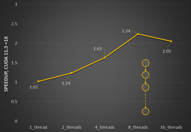
Figure showing the relative launch latency improvements in CUDA 11.4 for multithreaded launch of a straight-line graph for different numbers of threads.
Figure 2. Multithreaded launch latency improvement for a straight line for repeat launches with CUDA 11.3 baselines.

Stream-ordered memory allocator support

The stream-ordered memory allocator enables applications to order memory allocation and deallocation with respect to other work launched into a CUDA stream. This also enables allocation re-use, which can significantly improve application performance. For more information about the feature and capabilities, see Enhancing Memory Allocation with New NVIDIA CUDA 11.2 Features.

In CUDA 11.4, CUDA Graphs now supports stream-ordered memory allocation both through stream capture or in native graph construction through new allocate and free node types, enabling the same efficient, deferred memory reuse logic within graphs.

These node types are collectively referred to as memory nodes.  They can be created in several ways:

  • Using the explicit API
    • Using cudaGraphAddMemAllocNode and cudaGraphAddMemFreeNode, respectively
  • Using stream capture
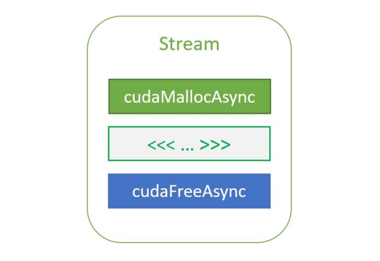
    • Using cudaMallocAsync/cudaMallocFromPoolAsync and cudaFreeAsync, respectively

In the same way that stream-ordered allocation uses implicit stream ordering and event dependencies to reuse memory, graph-ordered allocation uses the dependency information defined by the edges of the graph to do the same.
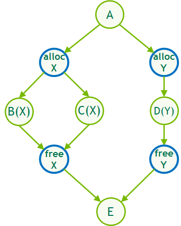
Figure showing the new Memalloc and MemFree graph nodes in a simple graph example
Figure 3. Intra-graph memory reuse. When a MemAlloc node is created, it attempts to reuse memory, which was freed by MemFree nodes that it depends upon.

For more information, see Stream Ordered Memory Allocator.

Enhancements to MPS

The Multi-Process Service (MPS) is a binary-compatible client-server runtime implementation of the CUDA API designed to transparently enable co-operative multiprocess CUDA applications.

It consists of a control daemon process, client runtime, and server process. MPS enables better GPU utilization in cases where a single process does not use all the compute and memory-bandwidth capacity. MPS also reduces on-GPU context storage and context switching. For more information, see Multi-Process Service in the GPU Management and Deployment guide.

In this release, we made a couple of key enhancements to improve the ease of use of MPS.
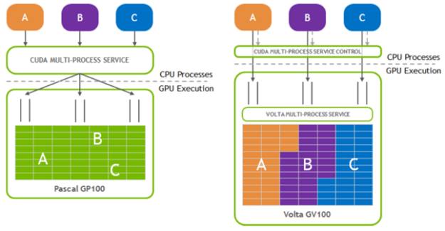
Figure showing the schematic representation of MPS on pre-Volta and post-Volta GPUs
Figure 4. Schematic representation of MPS with reduced on-GPU context storage and context switching to improve ease-of-use.

Programmatic configuration of SM partitions

There are certain use cases that share the following characteristics:

  • They consist of kernels that have little to no interaction, which enables concurrent execution.
  • The ratio of SMs required by these workloads may change and requires flexibility in allocating the right number of SMs.

The MPS active thread percentage setting enables you to limit the execution to a portion of the SMs. Before CUDA 11.4, this was a fixed value that was set equally for all clients within the process. In CUDA 11.4, this has been extended to offer a mechanism to partition the SMs at a per-client level through a programmatic interface. This enables you to create contexts that have different SM partitions within the same application process.

A new resource type called CU_EXEC_AFFINITY_TYPE_SM_COUNT enables you to specify a minimum number N that the context requires. The system guarantees that at least this many SMs are assigned, although more may be reserved. CUDA 11.4 also introduces a related affinity API cuCtxGetExecAffinity, which queries the exact amount of a resource (such as the SM count) allocated for a context. For more information, see the cuCtxGetExecAffinity section in the API documentation.

Error reporting

To improve the error reporting and ease of diagnosing the root cause of MPS issues, we introduced new and detailed driver and runtime error codes. These error codes provide more specificity regarding the type of error. They supplement the common MPS error codes with additional information to help you trace down the cause of the failures. Use these error codes in your applications with the error messages in the server log, as part of the root cause analysis.

New error codes:

 CUDA_ERROR_MPS_CONNECTION_FAILED
 CUDA_ERROR_MPS_SERVER_NOT_READY
 CUDA_ERROR_MPS_RPC_FAILURE
 CUDA_ERROR_MPS_MAX_CLIENTS_REACHED
 CUDA_ERROR_MPS_MAX_CONNECTIONS_REACHED 

Formalizing asynchronous data movement

In support of the asynchronous memory transfer operations, enabled by NVIDIA A100 GPU microarchitecture, in CUDA 11.4, we formalized and defined the asynchronous SIMT programming model. The asynchronous programming model defines the behavior and the APIs for C++ 20 barriers and cuda::memcpy_async on the GPU.

For more information about how you can use the asynchronous APIs to overlap memory operations from global memory, with computations in the streaming multiprocessors (SMs), see Asynchronous SIMT Programming Model.

Other enhancements

In addition to the key capabilities listed earlier, there are a few enhancements in CUDA 11.4 geared towards improving the mulit-thread submission throughput and extending the CUDA forward compatibility support to NVIDIA RTX GPUs.

Multithread submission throughput

In 11.4, we reduced the serialization of the CUDA API overheads between CPU threads. These changes are enabled by default. However, to assist with the triage of possible issues because of the underlying changes, we provide an environment variable, CUDA_REDUCE_API_SERIALIZATION, to turn off these changes. This was one of the underlying changes discussed earlier that contributed to the performance improvements for CUDA graphs.

CUDA forward compatibility

To enable use cases where you want to update your CUDA toolkit but stay on your current driver version, for example to reduce the risk or the overhead of additional validation needed to move to a new driver, CUDA offers the CUDA forward compatibility path. This was introduced in CUDA 10.0 but was initially limited to data-center GPUs. CUDA 11.4 eases those restrictions and you can now take advantage of the forward compatibility path for NVIDIA RTX GPUs as well.
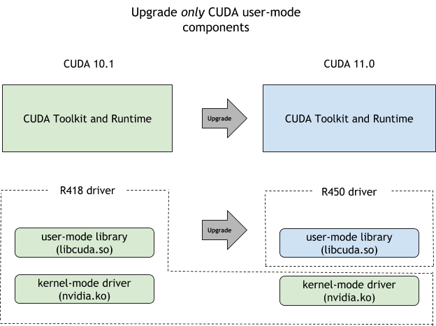
Figure showing flowchart diagram to help developers decide which CUDA driver upgrade path best meets their needs
Figure 5. Forward compatibility upgrade path between pre-CUDA 11.0 releases and current CUDA 11.x drivers.

C++ language support for CUDA

Here are some key enhancements included with C++ language support in CUDA 11.4.

  • Major releases:
    • NVIDIA C++ Standard Library (libcu++) 1.5.0 was released with CUDA 11.4.
    • Thrust 1.12.0 has the new thrust::universal_vector API that enables you to use the CUDA unified memory with Thrust.
  • Bug fix release: The CUDA 11.4 toolkit release includes CUB 1.12.0.
  • New asynchronous thrust::async:exclusive_scan and inclusive_scan algorithms have been added, and the synchronous versions of these were updated to use cub::DeviceScan directly.

CUDA compiler enhancements

CUDA 11.4 NVCC C++ compiler has JIT LTO support in preview, offers more L1 and L2 cache control, and exposes a C++ symbol demangling static library along with NVIDIA Nsight debugger support for alloca.

JIT link time optimization

JIT link-time optimization (LTO) is a preview feature and is available only on CUDA Toolkit 11.4, not on embedded platforms. This feature enables LTO to be performed at runtime. Use NVRTC to generate NVVM IR, and then use the cuLink driver APIs to link the NVVM IR and do LTO. 

The following code example shows how runtime JIT LTO can be used in your program.
Generate NVVM IR using nvrtcCompileProgram with the -dlto option and retrieve the generated NVVM IR using the newly introduced nvrtcGetNVVM.  Existing cuLink APIs are augmented to take newly introduced JIT LTO options to accept NVVM IR as input and to perform JIT LTO. Pass the CU_JIT_LTO option to cuLinkCreate API to instantiate the linker and then use CU_JIT_INPUT_NVVM as option to cuLinkAddFile or cuLinkAddData API for further linking of NVVM IR.

 nvrtcProgram prog1, prog2;
 CUlinkState linkState;
 int err;
 void* cubin;
 size_t cubinSize;
 char *nvvmIR1, *nvvmIR2;
 
 
 NVRTC_SAFE_CALL(
      nvrtcCompileProgram(&prog1, ...);
 NVRTC_SAFE_CALL(
      nvrtcCompileProgram(&prog2, ...);
 
 const char* opts = (“--gpu-architecture=compute_80”, “--dlto”);
 
 nvrtcGetNVVM(prog1, &nvvmIR1);
 nvrtcGetNVVM(prog1, &nvvmIR2);
  
  
 options[0] = CU_JIT_LTO;
 values[0] = (void*)&walltime;
 ...
 cuLinkCreate(..., options, values, &linkState);
 err = cuLinkAddData(linkState, CU_JIT_INPUT_NVVM,
                     (void*)nvvmIR1, strlen(nvvmIR1) + 1, ...);
 ...
 err = cuLinkAddData(linkState, CU_JIT_INPUT_NVVM,
                     (void*)nvvmIR2, strlen(nvvmIR2) + 1, ...);
 ...
 cuLinkComplete(linkState, &cubin, &cubinSize);
 ... 

Libcu++flt library support

The CUDA SDK now ships with libcu++filt, a static library that converts compiler-mangled C++  symbols into user-readable names. The following API, found in the nv_decode.h header file, is the entry point to the library:

char* __cu_demangle(const char* id, char *output_buffer, size_t *length, int *status) 

The following C++ example code shows usage:

 #include 
 #include "/usr/local/cuda-14.0/bin/nv_decode.h"
  
 using namespace std;
 int main(int argc, char **argv)
 {
   const char* mangled_name = "_ZN6Scope15Func1Enez";
   int status = 1;
   char* w = __cu_demangle(mangled_name,0,0,&status);
   if(status != 0)
     cout


This code example outputs as follows:

Demangling Succeeded: Scope1::Func1(__int128, long double, ...)

For more information, see Library Availability in the CUDA Binary Utilities documentation.

Configuring cache behavior in PTX

PTX ISA 7.4 gives you more control over caching behavior of both L1 and L2 caches. The following capabilities are introduced in this PTX ISA version:

  • Enhanced data prefetching: The new .level::prefetch_size qualifier can be used to prefetch additional data along with memory load or store operations. This enables exploiting the spatial locality of data.
  • Eviction priority control: PTX ISA 7.4 introduces four cache eviction priorities. These eviction priorities can be specified with the .level::eviction_priority qualifier on memory load or store operations (applicable to the L1 cache) and on the prefetch instruction (applicable to the L2 cache).
    • evict_normal (default)
    • evict_last (useful when the data should be kept in the cache longer)
    • evict_first (useful for streaming data)
    • no_allocate (avoid data from being cached at all)
  • Enhanced L2 cache control: This comes in two flavors:
    • Cache control on specific addresses: The new discard instruction enables discarding data from cache without writing it back to memory. It should be only used when the data is no longer required. The new applypriority instruction sets the eviction priority of specific data to evict_normal. This is [articularly useful in downgrading the eviction priority from evict_last when the data no longer needs to be persistent in cache.
    • Cache-hints on memory operations: The new createpolicy instruction enables creating a cache policy descriptor that encodes one or more cache eviction priorities for different data regions. Several memory operations including load, store, asynchronous copy, atom, red, and so on can accept cache policy descriptor as an operand when the .level::cache_hint qualifier is used.

These extensions are treated as performance hints only. The caching behavior specified using these extensions is not guaranteed by the caching system. For more information about usage, see the PTX ISA specification.

Other compiler enhancements in CUDA 11.4 include support for a new host compiler: ICC 2021. The diagnostics emitted by the CUDA frontend compiler are now ANSI colored and Nsight debugger can now correctly unwind CUDA applications with alloca calls, in the Call Stack view.

Nsight Developer Tools

New versions are now available for NVIDIA Nsight Visual Studio Code Edition (VSCE) and Nsight Compute 2021.2, adding enhancements to the developer experience for CUDA programming.

NVIDIA Nsight VSCE is an application development environment for heterogeneous platforms bringing CUDA development for GPUs into Microsoft Visual Studio Code. NVIDIA Nsight VSCE enables you to build and debug GPU kernels and native CPU code in the same session as well as inspect the state of the GPU and memory.

It includes IntelliSense code highlighting for CUDA applications and an integrated GPU debugging experience from the IDE with support for stepping through code, setting breakpoint, and inspecting memory states and system information in CUDA kernels. Now it’s easy to develop and debug CUDA applications directly from Visual Studio Code.

Nsight Compute 2021.2 adds new features that help detect more performance issues and make it easier to understand and fix them. The new register dependency visualization (Figure 6) helps identify long dependency chains and inefficient register usage that can limit performance. This release also adds a frequently requested feature to enable you to view the side-by-side assembly and correlated source code for CUDA kernels in the source view, without needing to collect a profile. This standalone source viewer feature enables you to open .cubin files directly from disk in the GUI to see the code correlation.
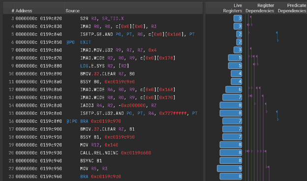
Example screen shot of Nsight Compute tool helping developers visualize registry dependency to help improve code performance
Figure 6. Nsight Compute Register Dependency Visualization capability helps identify long dependency chains and inefficient register usage to help improve performance.

Several features, including highlighted focus metrics, report cross-links, increased rule visibility, and documentation references all add to the built-in profile and optimization guided analysis that Nsight Compute provides to help you understand and fix performance bottlenecks.

This release also includes support for OptiX 7 resource tracking, a new Python interface for reading report data, and improvements to management of baseline reports, font settings, and CLI filters.

For overall updates, see NVIDIA Developer Tools Overview. Download the tools to your code.

For more information about the CUDA 11 generation toolkit capabilities and introductions, see CUDA 11 Features Revealed and follow all CUDA posts.

Acknowledgements

Thanks to the following key contributors: Stephen Jones, Arthy Sundaram, Fred Oh, and Sally Stevenson.
Categories
Misc

Using the NVIDIA CUDA Stream-Ordered Memory Allocator, Part 1

Most CUDA developers are familiar with the cudaMalloc and cudaFree API functions to allocate GPU accessible memory. However, there has long been an obstacle with these API functions: they aren’t stream ordered. In this post, we introduce new API functions, cudaMallocAsync and cudaFreeAsync, that enable memory allocation and deallocation to be stream-ordered operations. In part … Continued
Most CUDA developers are familiar with the cudaMalloc and cudaFree API functions to allocate GPU accessible memory. However, there has long been an obstacle with these API functions: they aren’t stream ordered. In this post, we introduce new API functions, cudaMallocAsync and cudaFreeAsync, that enable memory allocation and deallocation to be stream-ordered operations.

In part 2 of this series, we highlight the benefits of this new capability by sharing some big data benchmark results and provide a code migration guide for modifying your existing applications. We also cover advanced topics to take advantage of stream-ordered memory allocation in the context of multi-GPU access and the use of IPC. This all helps you improve performance within your existing applications.

Stream ordering efficiency

The following code example on the left is inefficient because the first cudaFree call has to wait for kernelA to finish, so it synchronizes the device before freeing the memory. To make this run more efficiently, the memory can be allocated upfront and sized to the larger of the two sizes, as shown on the right.

cudaMalloc(&ptrA, sizeA);
kernelA>>(ptrA);
cudaFree(ptrA); // Synchronizes the 
device before freeing memory
cudaMalloc(&ptrB, sizeB);
kernelB>>(ptrB);
cudaFree(ptrB);
cudaMalloc(&ptr,   max(sizeA, sizeB));
kernelA>>(ptr);
kernelB>>(ptr);
cudaFree(ptr); 

This increases code complexity in the application because the memory management code is separated out from the business logic. The problem is exacerbated when other libraries are involved. For example, consider the case where kernelA is launched by a library function instead:

libraryFuncA(stream);
cudaMalloc(&ptrB, sizeB);
kernelB>>(ptrB);
cudaFree(ptrB);
  
void libraryFuncA(cudaStream_t stream) {
    cudaMalloc(&ptrA, sizeA);
    kernelA>>(ptrA);
    cudaFree(ptrA);
 } 

This is much harder for the application to make efficient because it may not have complete visibility or control over what the library is doing. To circumvent this problem, the library would have to allocate memory when that function is invoked for the first time and never free it until the library is deinitialized. This not only increases code complexity, but it also causes the library to hold on to the memory longer than it needs to, potentially denying another portion of the application from using that memory.

Some applications take the idea of allocating memory upfront even further by implementing their own custom allocator. This adds a significant amount of complexity to application development. CUDA aims to provide a low-effort, high-performance alternative.

CUDA 11.2 introduced a stream-ordered memory allocator to solve these types of problems, with the addition of cudaMallocAsync and cudaFreeAsync. These new API functions shift memory allocation from global-scope operations that synchronize the entire device to stream-ordered operations that enable you to compose memory management with GPU work submission. This eliminates the need for synchronizing outstanding GPU work and helps restrict the lifetime of the allocation to the GPU work that accesses it. Consider the following code example:

cudaMallocAsync(&ptrA, sizeA, stream);
kernelA>>(ptrA);
cudaFreeAsync(ptrA, stream); // No synchronization necessary
cudaMallocAsync(&ptrB, sizeB, stream); // Can reuse the memory freed previously
kernelB>>(ptrB);
cudaFreeAsync(ptrB, stream); 

It is now possible to manage memory at function scope, as in the following example of a library function launching kernelA.

libraryFuncA(stream);
cudaMallocAsync(&ptrB, sizeB, stream); // Can reuse the memory freed by the library call
kernelB>>(ptrB);
cudaFreeAsync(ptrB, stream);
  
void libraryFuncA(cudaStream_t stream) {
    cudaMallocAsync(&ptrA, sizeA, stream);
    kernelA>>(ptrA);
    cudaFreeAsync(ptrA, stream); // No synchronization necessary
} 

Stream-ordered allocation semantics

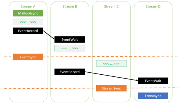
All the usual stream-ordering rules apply to cudaMallocAsync and cudaFreeAsync. The memory returned from cudaMallocAsync can be accessed by any kernel or memcpy operation as long as the kernel or memcpy is ordered to execute after the allocation operation and before the deallocation operation, in stream order. Deallocation can be performed in any stream, as long as it is ordered to execute after the allocation operation and after all accesses on all streams of that memory on the GPU.

In effect, stream-ordered allocation behaves as if allocation and free were kernels. If kernelA produces a valid buffer on a stream and kernelB invalidates it on the same stream, then an application is free to access the buffer after kernelA and before kernelB in the appropriate stream order.

The following example shows various valid usages.

auto err = cudaMallocAsync(&ptr, size, streamA);
// If cudaMallocAsync completes successfully, ptr is guaranteed to be
// a valid pointer to memory that can be accessed in stream order
  
assert(err == cudaSuccess);
  
// Work launched in the same stream can access the memory because 
// operations within a stream are serialized by definition
  
kernel>>(ptr);
  
// Work launched in another stream can access the memory as long as
// the appropriate dependencies are added
  
cudaEventRecord(event, streamA);
cudaStreamWaitEvent(streamB, event, 0);
kernel>>(ptr);
 
 
// Synchronizing the stream at a point beyond the allocation operation 
// also enables any stream to access the memory
  
cudaEventSynchronize(event);
kernel>>(ptr);
  
// Deallocation requires joining all the accessing streams. Here, 
// streamD will be deallocating.
// Adding an event dependency on streamB ensures that all accesses in 
// streamB will be done before the deallocation
  
cudaEventRecord(event, streamB);
cudaStreamWaitEvent(streamD, event, 0);
  
// Synchronizing streamC also ensures that all its accesses are done before 
// the deallocation
  
cudaStreamSynchronize(streamC);
cudaFreeAsync(ptr, streamD); 

Figure 1 shows the various dependencies specified in the earlier code example. As you can see, all kernels are ordered to execute after the allocation operation and complete before the deallocation operation.

Figure showing how to correctly access memory allocated using cudaMallocAsync.
Figure 1. Various ways to insert dependencies between streams to ensure correctness when accessing memory allocated using cudaMallocAsync.

Memory allocation and deallocation cannot fail asynchronously. Memory errors that occur because of a call to cudaMallocAsync or cudaFreeAsync (for example, out of memory) are reported immediately through an error code returned from the call. If cudaMallocAsync completes successfully, the returned pointer is guaranteed to be a valid pointer to memory that is safe to access in the appropriate stream order.

err = cudaMallocAsync(&ptr, size, stream);
if (err != cudaSuccess) {
    return err;
}
// Now you’re guaranteed that ‘ptr’ is valid when the kernel executes on stream
kernel>>(ptr);
cudaFreeAsync(ptr, stream); 

The CUDA driver uses memory pools to achieve the behavior of returning a pointer immediately.

Memory pools

The stream-ordered memory allocator introduces the concept of memory pools to CUDA. A memory pool is a collection of previously allocated memory that can be reused for future allocations. In CUDA, a pool is represented by a cudaMemPool_t handle. Each device has a notion of a default pool whose handle can be queried using cudaDeviceGetDefaultMemPool.

You can also explicitly create your own pools and either use them directly or set them as the current pool for a device and use them indirectly. Reasons for explicit pool creation include custom configuration, as described later in this post. When no explicitly created pool has been set as the current pool for a device, the default pool acts as the current pool.

When called without an explicit pool argument, each call to cudaMallocAsync infers the device from the specified stream and attempts to allocate memory from that device’s current pool. If the pool has insufficient memory, the CUDA driver calls into the OS to allocate more memory. Each call to cudaFreeAsync returns memory to the pool, which is then available for re-use on subsequent cudaMallocAsync requests. Pools are managed by the CUDA driver, which means that applications can enable pool sharing between multiple libraries without those libraries having to coordinate with each other.

If a memory allocation request made using cudaMallocAsync can’t be serviced due to fragmentation of the corresponding memory pool, the CUDA driver defragments the pool by remapping unused memory in the pool to a contiguous portion of the GPU’s virtual address space. Remapping existing pool memory instead of allocating new memory from the OS also helps keep the application’s memory footprint low.

By default, unused memory accumulated in the pool is returned to the OS during the next synchronization operation on an event, stream, or device, as the following code example shows.

cudaMallocAsync(ptr1, size1, stream); // Allocates new memory into the pool
kernel>>(ptr);
cudaFreeAsync(ptr1, stream); // Frees memory back to the pool
cudaMallocAsync(ptr2, size2, stream); // Allocates existing memory from the pool
kernel>>(ptr2);
cudaFreeAsync(ptr2, stream); // Frees memory back to the pool
cudaDeviceSynchronize(); // Frees unused memory accumulated in the pool back to the OS
// Note: cudaStreamSynchronize(stream) achieves the same effect here 

Retaining memory in the pool

Returning memory from the pool to the system can affect performance in some cases. Consider the following code example:

for (int i = 0; i >>(ptr);
    cudaFreeAsync(ptr, stream);
    cudaStreamSynchronize(stream);
}

By default, stream synchronization causes any pools associated with that stream’s device to release all unused memory back to the system. In this example, that would happen at the end of every iteration. As a result, there is no memory to reuse for the next cudaMallocAsync call and instead memory must be allocated through an expensive system call.

To avoid this expensive reallocation, the application can configure a release threshold to enable unused memory to persist beyond the synchronization operation. The release threshold specifies the maximum amount of memory the pool caches. It releases all excess memory back to the OS during a synchronization operation.

By default, the release threshold of a pool is zero. This means that allunused memory in the pool is released back to the OS during every synchronization operation. The following code example shows how to change the release threshold.

cudaMemPool_t mempool;
cudaDeviceGetDefaultMemPool(&mempool, device);
uint64_t threshold = UINT64_MAX;
cudaMemPoolSetAttribute(mempool, cudaMemPoolAttrReleaseThreshold, &threshold);
for (int i = 0; i >>(ptr);
    cudaFreeAsync(ptr, stream);
    cudaStreamSynchronize(stream);    // Only releases memory down to “threshold” bytes
} 

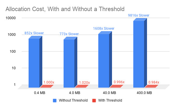
Using a nonzero release threshold enables reusing memory from one iteration to the next. This requires only simple bookkeeping and makes the performance of cudaMallocAsync independent of the size of the allocation, which results in dramatically improved memory allocation performance (Figure 2).

Figure showing differences in cost of memory allocation with and without a release threshold.
Figure 2. Cost of allocating memory using cudaMallocAsync with and without setting a release threshold (all values relative to performance of 0.4MB with threshold allocation).

The pool threshold is just a hint. Memory in the pool can also be released implicitly by the CUDA driver to enable an unrelated memory allocation request in the same process to succeed. For example, a call to cudaMalloc or cuMemCreate could cause CUDA to free unused memory from any memory pool associated with the device in the same process to serve the request.

This is especially helpful in scenarios where an application makes use of multiple libraries, some of which use cudaMallocAsync and some that do not. By automatically freeing up unused pool memory, those libraries do not have to coordinate with each other to have their respective allocation requests succeed.

There are limitations to when the CUDA driver automatically reassigns memory from a pool to unrelated allocation requests. For example, the application may be using a different interface, like Vulkan or DirectX, to access the GPU, or there may be more than one process using the GPU at the same time. Memory allocation requests in those contexts do not cause automatic freeing of unused pool memory. In such cases, the application may have to explicitly free unused memory in the pool, by invoking cudaMemPoolTrimTo.

size_t bytesToKeep = 0;
cudaMemPoolTrimTo(mempool, bytesToKeep); 

The bytesToKeep argument tells the CUDA driver how many bytes it can retain in the pool. Any unused memory that exceeds that size is released back to the OS.

Better performance through memory reuse

The stream parameter to cudaMallocAsync and cudaFreeAsync helps CUDA reuse memory efficiently and avoid expensive calls into the OS. Consider the following trivial code example.

cudaMallocAsync(&ptr1, size1, stream);
kernelA>>(ptr1);
cudaFreeAsync(ptr1, stream);
cudaMallocAsync(&ptr2, size2, stream);
kernelB>>(ptr2); 
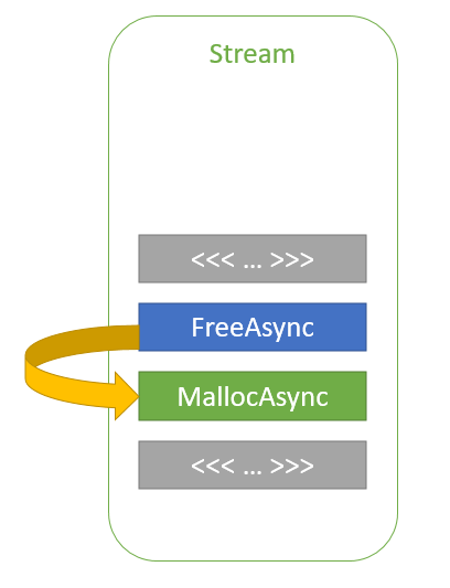
Figure showing how memory can be reused within a stream.
Figure 3. Memory reuse within the same stream.

In this code example, ptr2 is allocated in stream order after ptr1 is freed. The ptr2 allocation could reuse some, or all, of the memory that was used for ptr1 without any synchronization, because kernelA and kernelB are launched in the same stream. So, stream-ordering semantics guarantee that kernelB cannot begin execution and access the memory until kernelA has completed. This way, the CUDA driver can help keep the memory footprint of the application low while also improving allocation performance.

The CUDA driver can also follow dependencies between streams inserted through CUDA events, as shown in the following code example:

cudaMallocAsync(&ptr1, size1, streamA);
kernelA>>(ptr1);
cudaFreeAsync(ptr1, streamA);
cudaEventRecord(event, streamA);
cudaStreamWaitEvent(streamB, event, 0);
cudaMallocAsync(&ptr2, size2, streamB);
kernelB>>(ptr2); 
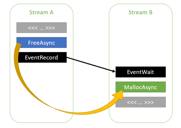
Figure showing how memory can be reused across dependent streams.
Figure 4. Memory reuse across streams with an event dependency between them.

As the CUDA driver is aware of the dependency between streams A and B, it can reuse the memory used by ptr1 for ptr2. The dependency chain between streams A and B can contain any number of streams, as shown in the following code example.

cudaMallocAsync(&ptr1, size1, streamA);
kernelA>>(ptr1);
cudaFreeAsync(ptr1, streamA);
cudaEventRecord(event, streamA);
for (int i = 0; i >>(ptr2); 

If necessary, the application can disable this feature on a per-pool basis:

int enable = 0;
cudaMemPoolSetAttribute(mempool, cudaMemPoolReuseFollowEventDependencies, &enable); 

The CUDA driver can also reuse memory opportunistically in the absence of explicit dependencies specified by the application. While such heuristics may help improve performance or avoid memory allocation failures, they can add nondeterminism to the application and so can be disabled on a per-pool basis. Consider the following code example:

cudaMallocAsync(&ptr1, size1, streamA);
kernelA>>(ptr1);
cudaFreeAsync(ptr1);
cudaMallocAsync(&ptr2, size2, streamB);
kernelB>>(ptr2);
cudaFreeAsync(ptr2); 

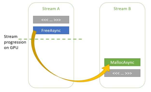
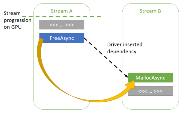
In this scenario, there are no explicit dependencies between streamA and streamB. However, the CUDA driver is aware of how far each stream has executed. If, on the second call to cudaMallocAsync in streamB, the CUDA driver determines that kernelA has finished execution on the GPU, then it can reuse some or all of the memory used by ptr1 for ptr2.

Figure showing how memory can be reused opportunistically across streams.
Figure 5. Opportunistic memory reuse across streams.

If kernelA has not finished execution, the CUDA driver can add an implicit dependency between the two streams such that kernelB does not begin executing until kernelA finishes.

Figure showing how memory can be reused across streams through implicit dependencies added by the CUDA driver.
Figure 6. Memory reuse through internal dependencies.

The application can disable these heuristics as follows:

int enable = 0;
cudaMemPoolSetAttribute(mempool, cudaMemPoolReuseAllowOpportunistic, &enable);
cudaMemPoolSetAttribute(mempool, cudaMemPoolReuseAllowInternalDependencies, &enable); 

Summary

In part 1 of this series, we introduced the new API functions cudaMallocAsync and cudaFreeAsync , which enable memory allocation and deallocation to be stream-ordered operations. Use them to avoid expensive calls to the OS through memory pools maintained by the CUDA driver.

In part 2 of this series, we share some benchmark results to show the benefits of stream-ordered memory allocation. We also provide a step-by-step recipe for modifying your existing applications to take full advantage of this advanced CUDA capability.

Categories
Misc

How Was NVIDIA’s 2021 GTC Keynote Made? Step Inside Our Kitchen Aug. 11 to Find Out

Ever see a virtual kitchen materialize in real-time? If you caught NVIDIA CEO Jensen Huang’s keynote for our March 2021 GPU Technology Conference you’re no doubt wondering about more than a few of the presentation’s magic tricks. With the premiere of “Connecting in the Metaverse: The Making of the GTC Keynote,” Wednesday, Aug. 11, at Read article >

The post How Was NVIDIA’s 2021 GTC Keynote Made? Step Inside Our Kitchen Aug. 11 to Find Out appeared first on The Official NVIDIA Blog.

Categories
Misc

Using the NVIDIA CUDA Stream-Ordered Memory Allocator, Part 2

In part 1 of this series, we introduced new API functions, cudaMallocAsync and cudaFreeAsync, that enable memory allocation and deallocation to be stream-ordered operations. In this post, we highlight the benefits of this new capability by sharing some big data benchmark results and provide a code migration guide for modifying your existing applications. We also … Continued

In part 1 of this series, we introduced new API functions, cudaMallocAsync and cudaFreeAsync, that enable memory allocation and deallocation to be stream-ordered operations. In this post, we highlight the benefits of this new capability by sharing some big data benchmark results and provide a code migration guide for modifying your existing applications. We also cover advanced topics to take advantage of stream-ordered memory allocation in the context of multi-GPU access and the use of IPC. This all helps you improve performance within your existing applications.

GPU Big Data Benchmark

To measure the performance impact of the new stream-ordered allocator in a real application, here are results from the RAPIDS GPU Big Data Benchmark (gpu-bdb). gpu-bdb is a benchmark of 30 queries representing real-world data science and machine learning workflows at various scale factors: SF1000 is 1 TB of data and SF10000 is 10 TB. Each query is, in fact, a model workflow that can include SQL, user-defined functions, careful subsetting and aggregation, and machine learning.

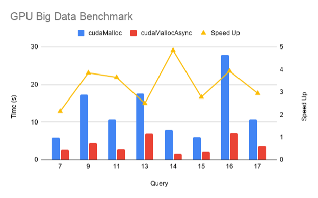
Figure 1 shows the performance of cudaMallocAsync compared to cudaMalloc for a subset of gpu-bdb queries conducted at SF1000 on an NVIDIA DGX-2 across 16 V100 GPUs. As you can see, thanks to memory reuse and eliminating extraneous synchronization, there’s a 2–5x improvement in end-to-end performance when using cudaMallocAsync.

Figure showing the performance improvement using stream-ordered memory allocation API functions in the GPU big data benchmark.
Figure 1. Speed up of cudaMallocAsync over cudaMalloc for various queries on the RAPIDS GPU Big Data Benchmark.

Interoperability with cudaMalloc and cudaFree

An application can use cudaFreeAsync to free a pointer allocated by cudaMalloc. The underlying memory is not freed until the next synchronization of the stream passed to cudaFreeAsync.

cudaMalloc(&ptr, size);
kernel>>(ptr);
cudaFreeAsync(ptr, stream);
cudaStreamSynchronize(stream); // The memory for ptr is freed at this point 

Similarly, an application can use cudaFree to free memory allocated using cudaMallocAsync. However, cudaFree does not implicitly synchronize in this case, so the application must insert the appropriate synchronization to ensure that all accesses to the to-be-freed memory are complete. Any application code that may be intentionally or accidentally relying on the implicit synchronization behavior of cudaFree must be updated.

cudaMallocAsync(&ptr, size, stream);
kernel>>(ptr);
cudaStreamSynchronize(stream); // Must synchronize first
cudaFree(ptr);

Multi-GPU access

By default, memory allocated using cudaMallocAsync is accessible from the device associated with the specified stream. Accessing the memory from any other device requires enabling access to the entire pool from that other device. It also requires the two devices to be peer capable, as reported by cudaDeviceCanAccessPeer. Unlike cudaMalloc allocations, cudaDeviceEnablePeerAccess and cudaDeviceDisablePeerAccess have no effect on memory allocated from memory pools.

For example, consider enabling device 4access to the memory pool of device 3:

cudaMemPool_t mempool;
cudaDeviceGetDefaultMemPool(&mempool, 3);
cudaMemAccessDesc desc = {};
desc.location.type = cudaMemLocationTypeDevice;
desc.location.id = 4;
desc.flags = cudaMemAccessFlagsProtReadWrite;
cudaMemPoolSetAccess(mempool, &desc, 1 /* numDescs */); 

Access from a device other than the device on which the memory pool resides can be revoked by using cudaMemAccessFlagsProtNone when calling cudaMemPoolSetAccess. Access from the memory pool’s own device cannot be revoked.

Interprocess communication support

Memory allocated using the default memory pool associated with a device cannot be shared with other processes. An application must explicitly create its own memory pools to share memory allocated using cudaMallocAsync with other processes. The following code sample shows how to create an explicit memory pool with interprocess communication (IPC) capabilities:

cudaMemPool_t exportPool;
cudaMemPoolProps poolProps = {};
poolProps.allocType = cudaMemAllocationTypePinned;
poolProps.handleTypes = cudaMemHandleTypePosixFileDescriptor;
poolProps.location.type = cudaMemLocationTypeDevice;
poolProps.location.id = deviceId;
cudaMemPoolCreate(&exportPool, &poolProps); 

The location type Device and location ID deviceId indicate that the pool memory must be allocated on a specific GPU. The allocation type Pinned indicates that the memory should be non-migratable, also known as non-pageable. The handle type PosixFileDescriptor indicates that the user intends to query a file descriptor for the pool to share it with another process.

The first step to share memory from this pool through IPC is to query the file descriptor that represents the pool:

int fd;
cudaMemAllocationHandleType handleType = cudaMemHandleTypePosixFileDescriptor;
cudaMemPoolExportToShareableHandle(&fd, exportPool, handleType, 0); 

The application can then share the file descriptor with another process, for example through a UNIX domain socket. The other process can then import the file descriptor and obtain a process-local pool handle:

cudaMemPool_t importPool;
cudaMemAllocationHandleType handleType = cudaMemHandleTypePosixFileDescriptor;
cudaMemPoolImportFromShareableHandle(&importPool, &fd, handleType, 0); 

The next step is for the exporting process to allocate memory from the pool:

cudaMallocFromPoolAsync(&ptr, size, exportPool, stream); 

There is also an overloaded version of cudaMallocAsync that takes the same arguments as cudaMallocFromPoolAsync:

cudaMallocAsync(&ptr, size, exportPool, stream); 

After memory is allocated from this pool through either of these two APIs, the pointer can then be shared with the importing process. First, the exporting process gets an opaque handle representing the memory allocation:

cudaMemPoolPtrExportData data;
cudaMemPoolExportPointer(&data, ptr); 

This opaque data can then be shared with the importing process through any standard IPC mechanism, such as through shared memory, pipes, and so on The importing process then converts the opaque data into a process-local pointer:

cudaMemPoolImportPointer(&ptr, importPool, &data); 

Now both processes share access to the same memory allocation. The memory must be freed in the importing process before it is freed in the exporting process. This is to ensure that the memory does not get reutilized for another cudaMallocAsync request in the exporting process while the importing process is still accessing the previously shared memory allocation, potentially causing undefined behavior.

The existing function cudaIpcGetMemHandle works only with memory allocated through cudaMalloc and cannot be used on any memory allocated through cudaMallocAsync, regardless of whether the memory was allocated from an explicit pool.

Changing a device pool

If the application expects to use an explicit memory pool most of the time, it can consider setting that as the current pool for the device through cudaDeviceSetMemPool. This enables the application to avoid having to specify the pool argument each time that it must allocate memory from that pool.

cudaDeviceSetMemPool(device, pool);
cudaMallocAsync(&ptr, size, stream); // This now allocates from the earlier pool set instead of the device’s default pool. 

This has the advantage that any other function allocating with cudaMallocAsync now automatically uses the new pool as its default. The current pool associated with a device can be queried using cudaDeviceGetMemPool.

Library composability

In general, libraries should not change a device’s pool, as doing so affects the entire top-level application. If a library must allocate memory with different properties than those of the default device pool, it may create its own pool and then allocate from that pool using cudaMallocFromPoolAsync. The library could also use the overloaded version of cudaMallocAsync that takes the pool as an argument.

To make interoperability easier for applications, libraries should consider providing APIs for the top-level application to coordinate the pools used. For example, libraries could provide set or get APIs to enable the application to control the pool in a more explicit manner. The library could also take the pool as a parameter to individual APIs.

Code migration guide

When porting an existing application that uses cudaMalloc or cudaFree to the new cudaMallocAsync or cudaFreeAsync APIs, consider the following guidelines.

Guidelines for determining the appropriate pool:

  • The initial default pool is suitable for many applications.
  • Today, an explicitly constructed pool is only required to share pool memory across processes with CUDA IPC. This may change with future features.
  • For convenience, consider making the explicitly created pool the device’s current pool to ensure that all cudaMallocAsync calls within the process use that pool. This must be done by the top-level application and not by libraries, so as to avoid conflicting with the goals of the top-level application.

Guidelines for setting the release threshold for all memory pools:

  • The choice of release threshold depends on whether and how a device is shared:
    • Exclusive to a single process: Use the maximum release threshold.
    • Shared among cooperating processes: Coordinate to use the same pool through IPC or set each process pool to an appropriate value to avoid any one process monopolizing all device memory.
    • Shared among unknown processes: If known, set the threshold to the working set size of the application. Otherwise, leave it at zero and use a profiler to determine whether allocation performance is a bottleneck before using a nonzero value.

Guidelines for replacing cudaMalloc with cudaMallocAsync:

  • Ensure that all memory accesses are ordered after the stream-ordered allocation.
  • If peer access is required, use cudaMemPoolSetAccess as cudaEnablePeerAccess and cudaDisablePeerAccesss have no effect on pool memory.
  • Unlike cudaMalloc allocations, cudaDeviceReset does not implicitly free pool memory, so it must be explicitly freed.
  • If freeing with cudaFree, ensure that all accesses are complete through appropriate synchronization before freeing, as there is no implicit synchronization in this case. Any subsequent code that relied on the implicit synchronization may also have to be updated.
  • If memory is shared with another process through IPC, allocate from an explicitly created pool with IPC support and remove all references to cudaIpcGetMemHandle, cudaIpcOpenMemHandle, and cudaIpcCloseMemHandle for that pointer.
  • If the memory must be used with GPUDirect RDMA, continue to use cudaMalloc for now because memory allocated through cudaMallocAsync currently does not support it. CUDA aims to support this in the future.
  • Unlike memory allocated with cudaMalloc, memory allocated with cudaMallocAsync is not associated with a CUDA context. This has the following implications:
    • Calling cuPointerGetAttribute with the attribute CU_POINTER_ATTRIBUTE_CONTEXT returns null for the context.
    • When calling cudaMemcpy with at least one of source or destination pointers allocated using cudaMallocAsync, that memory must be accessible from the calling thread’s current context/device. If it’s not accessible from that context or device, use cudaMemcpyPeer instead.

Guidelines for replacing cudaFree with cudaFreeAsync:

  • Ensure that all memory accesses are ordered before the stream-ordered deallocation.
  • The memory may not be freed back to the system until the next synchronization operation. If the release threshold is set to a nonzero value, the memory may not be freed back to the system until the corresponding pool is explicitly trimmed.
  • Unlike cudaFree, cudaFreeAsync does not implicitly synchronize the device. Any code relying on this implicit synchronization must be updated to synchronize explicitly.

Conclusion

The stream-ordered allocator and cudaMallocAsync and cudaFreeAsync API functions added in CUDA 11.2 extend the CUDA stream programming model by introducing memory allocation and deallocation as stream-ordered operations. This enables allocations to be scoped to the kernels, which use them while avoiding costly device-wide synchronization that can occur with traditional cudaMalloc/cudaFree.

Furthermore, these API functions add the concept of memory pools to CUDA, enabling the reuse of memory to avoid costly system calls and improve performance. Use the guidelines to migrate your existing code and see how much your application performance improves!

Categories
Misc

Self supervision using tensorflow and keras

I have a self supervised problem, where I have a sequence of web page visits, each of which is denoted by some hash, and I can lookup this has to find a dense vector to represent this page.

I would like to train my model on various self supervised tasks, such as predicting a target page vector, given some context, or predicting the next vector in the sequence.

My question here is what is the best approach for implementation of such a problem? The naive approach would be to prep the data in a separate script.

I feel there must be a better approach, possibly using `tf.data.map` within the pipeline?

Would love to hear some best practices for self supervision, and the creation of datasets using TF and Keras.

submitted by /u/ydennisy
[visit reddit] [comments]

Categories
Misc

Using the MNIST database to recognize numbers

Im trying to use the MNIST database of handwritten numbers to make a neural network that predicts a number. The issue is that the validation accuracy is very high, around 98%, but when i try to apply the model to numbers outside of the database, the accuracy is very low. I got an accuracy of 50% with a dense network and 60% with a CNN. Im not sure what the issue is or how I can make the network work more consistently with new data that I give it. Any advice would be appreciated. If needed, I can send the code and test images.

submitted by /u/UnreadyDog
[visit reddit] [comments]

Categories
Misc

Upcoming DL RecSys Summit: Develop and Optimize Deep Learning Recommender Systems

The NVIDIA, Facebook, and TensorFlow recommender teams will be hosting a summit with live Q&A to dive into best practices and insights on how to develop and optimize deep learning recommender systems.

The NVIDIA, Facebook, and TensorFlow recommender teams will be hosting a summit with live Q&A to dive into best practices and insights on how to develop and optimize deep learning recommender systems.

Develop and Optimize Deep Learning Recommender Systems
Thursday, July 29 at 10 a.m. PT

By joining this Deep Learning Recommender Summit, you will hear from fellow ML engineers and data scientists from NVIDIA, Facebook, and TensorFlow on best practices, learnings, and insights for building and optimizing highly effective DL recommender systems.

Sessions include:

High-Performance Recommendation Model Training at Facebook
In this talk, we will first analyze how model architecture affects the GPU performance and efficiency, and also present the performance optimizations techniques we applied to improve the GPU utilization, which includes optimized PyTorch-based training stack supporting both model and data parallelism, high-performance GPU operators, efficient embedding table sharding, memory hierarchy and pipelining.

RecSys2021 Challenge: Predicting User Engagements with Deep Learning Recommender Systems
The NVIDIA team, a collaboration of Kaggle Grandmaster and NVIDIA Merlin, won the RecSys2021 challenge. It was hosted by Twitter, who provided almost 1 billion tweet-user pairs as a dataset. The team will present their winning solution with a focus on deep learning architectures and how to optimize them.

Revisiting Recommender Systems on GPU
A new era of faster ETL, Training, and Inference is coming to the RecSys space and this talk will walk through some of the patterns of optimization that guide the tools we are building to make recommenders faster and easier to use on the GPU.

TensorFlow Recommenders
TensorFlow Recommenders is an end-to-end library for recommender system models: from retrieval, through ranking, to post-ranking. In this talk, we describe how TensorFlow Recommenders can be used to fit and safely deploy sophisticated recommender systems at scale.

Register now >>

Categories
Misc

Accelerating Volkswagen Connected Car Data Pipelines 100x Faster with NVIDIA RAPIDS

Connected cars are vehicles that communicate with other vehicles using backend systems to enhance usability, enable convenient services, and keep distributed software maintained and up to date. At Volkswagen, we are working on connected car with NVIDIA to solve the challenges which have computational inefficiencies like Geospatial Indexing and K-Nearest Neighbors when implemented in native … Continued

Connected cars are vehicles that communicate with other vehicles using backend systems to enhance usability, enable convenient services, and keep distributed software maintained and up to date.

At Volkswagen, we are working on connected car with NVIDIA to solve the challenges which have computational inefficiencies like Geospatial Indexing and K-Nearest Neighbors when implemented in native python and pandas. 

Processing driving and sensor data is critical for connected cars to understand their environment. It enables connected cars to perform tasks such as parking spot detection, location-based services, theft protection, route recommendation through real-time traffic, fleet management, and many more. Location information is key to most of these use cases and requires a fast processing pipeline to enable real-time services. 

Global sales of connected cars are increasing rapidly, in turn, increasing the amount of data available. As per Gartner, the average connected vehicle will generate 280 petabytes of data annually, with four terabytes of data being generated in a day at the very least. The research also states that around 470 million connected vehicles will be deployed by 2025. 

This blog post will focus on the data pipeline required to process location-based geospatial information and deliver necessary services for connected cars. 

Challenges with connected cars data

Working with connected car data poses both technical and business challenges:

Fast processing of huge amounts of streaming data is needed because users expect a near real-time experience to make timely decisions. For example, if a user requests a parking spot and the system takes five minutes to respond, it’s likely the spot will already be taken by the time it answers. Faster processing and analyzing of the data is the key factor to overcome this challenge.

There are also data privacy issues to consider. Connected cars must satisfy the General Data Protection Regulation (GDPR). In short, GDPR requires that after data analysis, there should not be a chance to identify individual users from the analyzed data. Additionally, storage of data pertaining to individual users is prohibited (unless written consent is given by the user). Anonymization can meet these requirements by either masking the data that identifies the individual user or by grouping and aggregating the data so that traces of the user are not possible. For this purpose, we need to make sure that the software processing connected car data complies with the regulations required by GDPR on data anonymization, which adds additional compute requirements during the data processing.

A picture with three cars streaming data into cloud.
Figure 1: Schematic representation of connected cars data challenges.

Taking a data science approach

RAPIDS can address both the technical and business challenges of connected cars. The RAPIDS suite of open-source software (OSS) libraries and APIs gives you the ability to execute end-to-end data science and analytics pipelines entirely on GPUs. Licensed under Apache 2.0, RAPIDS was incubated by NVIDIA and based on extensive hardware and data science experience. RAPIDS utilizes NVIDIA CUDA primitives for low-level compute optimization and exposes GPU parallelism and high-bandwidth memory speed through user-friendly Python interfaces.

In the following sections, we discuss how RAPIDS (software) and NVIDIA GPUs (hardware) help tackle both the technical and business challenges on a prototype application using test data. Two different approaches will be evaluated, geospatial indexing and k-nearest neighbors.

Using RAPIDS, we are able to achieve a 100x speedup for this pipeline.

A brief introduction to geospatial indexing

Geospatial indexing is the basis for many algorithms in the domain of connected cars. It is the process of partitioning areas of the earth into identifiable grid cells. It is an effective way to prune the search space when querying the huge amount of data produced by connected cars.

Popular approaches include Military Grid Reference System (MGRS) and Uber’s Hexagonal Hierarchical Spatial Index (Uber H3).

In this data pipeline example, we use Uber H3 to split the records spatially into a set of smaller subsets.

The following are the conditions, which need to be satisfied after splitting the records into subsets:

  • Each subset consists of a maximum of ‘N’ records. This ‘N’ is chosen based on computational capacity constraints. For this experiment, we consider ‘N’ equals 2500 records.
  • The subset is denoted by subset_id, which is an auto-increment number starting from 0.

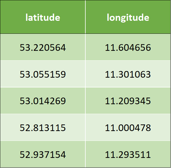
The following is the sample input data, which has two columns – latitude and longitude:

A table containing a sample of the input data. It consists of two columns: latitude and longitude.
Table 1: Sample input data.

The following is the algorithm that needs to be implemented to apply Uber H3 for the use case

  • Iterate over latitude and longitude, and assign hex_id from resolution 0.
  • If found any hex_id comprising less than 2500 records, then assign subset_id incrementally starting from 0.
  • Identify the hex_ids that comprise more than 2500 records.
  • Split the preceding records with an incremental resolution, which is now 1.
  • Repeat steps 3 and 4, until all the records are assigned to subset_id & hex_id or until the resolution reaches 15.

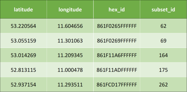
Once the preceding algorithm is applied, it results to the following output data:

Table 2: Sample output data after applying geospatial indexing.

Code snippets of Uber H3 implementation

Following is the code snippet of the implementation of Uber H3 using pandas:

#while loop until all the records are assigned to subset_id
while resolution  16 and df["subset_id"].isnull().any():
     #assignment of hex_id
     df['hex_id']= df.apply(lambda row: h3.geo_to_h3(row["latitude"],
                   row["longitude"], resolution), axis = 1)
      df_aggreg = df.groupby(by = "hex_id").size().reset_index()
     df_aggreg.columns = ["hex_id", "value"]
      #filtering the records that are less than 2500 count    
     hex_id = df_aggreg[df_aggreg['value']2500]['hex_id']
      #assignment of subset_id
     for index, value in hex_id.items():
         df.loc[df['hex_id'] == value, 'subset_id'] = subset_id
         subset_id += 1     
     df_return = df_return.append(df[~df['subset_id'].isna()],
                 ignore_index=True)
     df = df[df['subset_id'].isna()]
     resolution += 1

Following is the code snippet of the implementation of Uber H3 using PySpark:

#while loop until all the records are assigned to subset_id
while resolution  16 and (len(df.head(1)) != 0):
      #assignment of hex_id
     df = df.rdd.map(lambda x: (x["latitude"], x["longitude"],
          x["subset_id"],h3.geo_to_h3(x["latitude"], x["longitude"],
          resolution)))
      df = sqlContext.createDataFrame(df, schema)
     df_aggreg = df.groupby("hex_id").count()        
     df_aggreg = df_aggreg.withColumnRenamed("hex_id", "hex_id"
          .withColumnRenamed("count", "value")
      #filtering the records that are less than 2500 count
     hex_id = df_aggreg.filter(df_aggreg.value  2500)         
     var_hex_id = list(hex_id.select('hex_id').toPandas()['hex_id'])
     for i in var_hex_id:
         #assignment of subset_id
         df = df.withColumn('subset_id',F.when(df.hex_id==i,subset_id)
             .otherwise(df.subset_id)).select(df.latitude, df.longitude,
             'subset_id', df.hex_id)
          subset_id += 1
      df_return = df_return.union(df.filter(df.subset_id != 0))         
     df = df.filter(df.subset_id == 0)
     resolution += 1

With this pandas implementation of the Uber H3 model, we have identified a painfully slow execution. The slow execution of the code leads to significantly reduced productivity, as only little experiments can be done. The tangible goal is to speed up the execution time by 10x.

To accelerate the pipeline, we follow a step-by-step approach as follows. 

Step 1: Simple CPU parallel version

The idea of this version is to implement a simple multiprocessing-based kernel for the H3 library processing. The second part of the processing, which is assigning subsets according to the data, is the pandas library function, which cannot be easily parallelized.

#Function to assign hex_id
def minikernel(df, resolution):
 df['hex_id'] = np.vectorize(lambda latitude, longitude:
                 h3.geo_to_h3(latitude, longitude, resolution))(
                 np.array(df['latitude']), np.array(df['longitude']))
  return df
#while loop until all the records are assigned to subset_id
while resolution  16 and df["subset_id"].isnull().any():     
     #CPU Parallelization
     df_chunk = np.array_split(df, n_cores)
     pool = Pool(n_cores)
 
     #assigning hex_id by calling the function minikernel()
     df_chunk_res=pool.map(partial(minikernel, resolution=resolution),
                     df_chunk)
 
     df = pd.concat(df_chunk_res)
 
     pool.close()
     pool.join()
             
     df_aggreg = df.groupby(by = "hex_id").size().reset_index()
     df_aggreg.columns = ["hex_id", "value"]
     
     #filtering the records that are less than 2500 count
     hex_id = df_aggreg[df_aggreg['value']2500]['hex_id']
 
     for index, value in hex_id.items():
            #assignment of subset_id is pandas library function
            #which cannot be parallelized
         df.loc[df['hex_id'] == value, 'subset_id'] = subset_id
         subset_id += 1
    
     df_return = df_return.append(df[~df['subset_id'].isna()],
                 ignore_index=True)
 
     df = df[df['subset_id'].isna()]     
     resolution +=

By applying simple parallelization with a thread pool, we can significantly reduce the first part of the code (H3 library), but the second part (pandas library) is completely single-threaded and extremely slow.

Step 2: Apply RAPIDS cuDF 

The idea here is to use as many standard features from cuDF as possible (hence, the slightest code change) to achieve the best performance. As cuDF now operates on CUDA unified memory, it is not simply possible to parallelize the 1st part (H3 library) as cuDF does not handle CPU partitioning. The code is shown below. Note, the following code operates on a cuDF dataframe.

#while loop until all the records are assigned to subset_id
while resolution  16 and df["subset_id"].isnull().any():
     #assignment of hex_id
     #df is a cuDF
     df['hex_id'] = np.vectorize(lambda latitude, longitude:
                     h3.geo_to_h3(latitude, longitude, resolution))
                     (df['latitude'].to_array(), df['longitude']
                     .to_array())
     
     df_aggreg = df.groupby('hex_id').size().reset_index()
     df_aggreg.columns = ["hex_id", "value"]
 
     #filtering the records that are less than 2500 count
     hex_id = df_aggreg[df_aggreg['value']2500]['hex_id']
             
     for index, value in hex_id.to_pandas().items():
         #assignment of subset_id
         df.loc[df['hex_id'] == value, 'subset_id'] = subset_id
         subset_id += 1
         
     df_return = df_return.append(df[~df['subset_id'].isna()],
                 ignore_index=True)
 
     df = df[df['subset_id'].isna()]
     
     resolution += 1

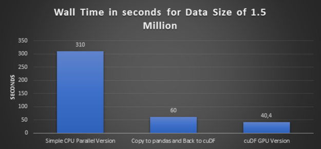
Step 3: Executing simple CPU parallelism version and cuDF GPU version using larger data

In this step, we increase the data volume three times, from half a million records to 1.5 million records, and execute a simple CPU parallel version and its equivalent cuDF GPU version.

Step 4: One more experiment with a copy to pandas and back to cuDF

As discussed in step 2, cuDF operates on CUDA-unified memory and it is not possible to parallelize the first part (H3 library) due to the lack of CPU-partitioning of the cuDF. Therefore, we have not used the function array_split. To overcome this challenge, first, we converted cuDF to pandas data frame, then applied the function array_split and then converted back the split chunk to cuDF and proceeded further with H3 library processing.

#while loop until all the records are assigned to subset_id
while resolution  16 and df["subset_id"].isnull().any():
     #copy to pandas
     df_temp = df.to_pandas()
     
     #CPU Parallelization
     df_chunk = np.array_split(df_temp, n_cores)
     pool = Pool(n_cores)
     df_chunk_res=pool.map(partial(minikernel, resolution=resolution),
                     df_chunk)
 
     pool.close()
     pool.join()
     
     df_temp = pd.concat(df_chunk_res)
     
     #Back to cuDF
     df = cudf.DataFrame(df_temp)
 
     #assignment of hex_id
     df['hex_id'] = np.vectorize(lambda latitude, longitude:
                     h3.geo_to_h3(latitude, longitude, resolution))
                     (df['latitude'].to_array(), df['longitude']
                     .to_array())
    
     df_aggreg = df.groupby('hex_id').size().reset_index()
     df_aggreg.columns = ["hex_id", "value"]
 
     #filtering the records that are less than 2500 count
     hex_id = df_aggreg[df_aggreg['value']2500]['hex_id']
             
     for index, value in hex_id.to_pandas().items():
         #assignment of subset_id
         df.loc[df['hex_id'] == value, 'subset_id'] = subset_id
         subset_id += 1
         
     df_return = df_return.append(df[~df['subset_id'].isna()],
                 ignore_index=True)
 
     df = df[df['subset_id'].isna()]
    
     resolution += 1 

Glancing graph with execution times over all the preceding approaches: 

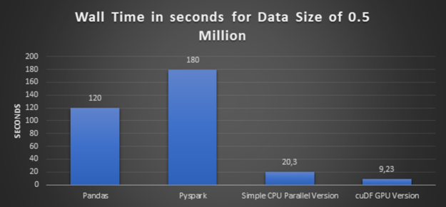
Figure 2: Execution times for various approaches with data size of 0.5 million.
Figure 3: Execution times for various approaches with data size of 1.5 million.

Lessons learned on speed-up geospatial index computation

  • High-Performance: The conclusion from the preceding glancing graphs is clear that cuDF GPU version delivers the best performance. And also bigger the dataset is, bigger the speedup is.
  • Code Adaptability and Easy Transition: Please notice that the code being ported is not the best scenario for GPU acceleration. We are running the comparison on a third-party library (Uber H3) which runs on CPU. To make use of that library, we need to copy the data from GPU memory to CPU memory on each loop, which is not the optimal approach.
    In addition to that, there is a subset_id calculation that is also done in a row-wise approach, which could potentially be speeded up by changing the original code. But still, the code is not changed because one of our main targets is to check code adaptability and easy transition between the libraries pandas and cuDF.
  • Reusable Code: As you had already observed from the preceding that the pipeline is a set of standardized functions and can just be used as functions to solve other use cases too.

Working towards a CUDA accelerated K-Nearest Neighbors (KNN) classification

Rather than measuring the density of connected cars by means of indexing and grouping, using the scheme above – another way is to perform geographical classification based on the earth distance between two locations.

The classification algorithm of our choice is K-Nearest Neighbors. The principle behind nearest neighbor methods is to find a predefined number of data points (K) closest in distance to the data point. We will be comparing a CPU-based implementation of KNN to the RAPIDS GPU-accelerated version of the same algorithm.

In our current use case, we work with anonymized streamed connected car data (as shortly described in business challenges preceding). Here, grouping and aggregating data using KNN is opted as part of anonymization.

However, for our use case, as we are grouping and aggregating on Geo-Coordinates, we will be using Haversine metric, which is the only metric that can cluster Geo-Coordinates.

In our pipeline inputs to KNN using haversine as distance metric will be the geo-coordinates (latitude, longitude) and the number of desired closest data points. In the example below, K = 7 was to be created.

In the following, we showcase the example with the same data in tuples (longitude and latitude).

  • Input data are the same tuples (longitude and latitude) as shown in the previous example.
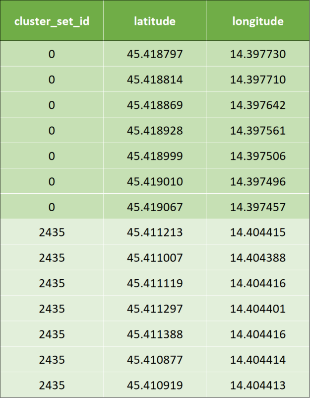
  • Once KNN is applied, a cluster id is calculated by the KNN algorithm: The clustered output data looks like below for the first two rows of input data. To avoid confusion, we marked the cluster ids with corresponding colors.
A table containing the output data after applying k-nearest neighbors classification to sample input data. It consists of four columns: custer_set_id, latitude and longitude.
Table 3: Sample output data after applying k-nearest neighbors classification.

Following is the code snippet of the implementation of KNN using pandas:

nbrs = NearestNeighbors(n_neighbors=7, algorithm='ball_tree',
     metric = "haversine").fit(coord_array_rad)
 
distances, indices = nbrs.kneighbors(coord_array_rad)
 
# Distance is computed in radians from haversine
distances_m = earth_radius * distances
 
# Drop KNN, which are not compliant with minimum distance
compliant_distances_mask = (distances_mKNN_MAX_DISTANCE)
                         .all(axis = 1)
 
compliant_indices = indices[compliant_distances_mask]

KNN is used as a classification algorithm. Drawback of KNN is its computational performance, especially when the data size is large. Our intention is to finally leverage cuML´s KNN implementation.

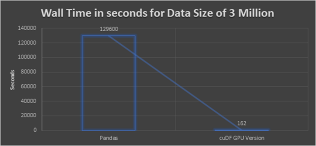
Preceding implementation worked in pretty small datasets but did not finish processing 3 million records within 1.5 days. Thus we stopped it.

In order to turn towards the CUDA accelerated KNN implementation, we had to mimic the haversine distance with an equivalent metric as shown below.

Step 1: Coordinate transformation to work around Haversine

At the moment of running this exercise, haversine distance metric was not available natively in cuML’s KNN implementation. Therefore, euclidean distance was used instead. Nevertheless, it is fair to mention that the current version of RAPIDS KNN already supports haversine metrics.

First of all, we converted the coordinates into the distance in meters in order to perform a distancing metric calculation. [10] This is implemented through a function named df_geo(), which will be used in the next step.

One caveat of Euclidean distance is that it does not work on coordinates on earth that are further distanced. Rather, it will basically “dig a hole” into the earth’s surface instead of being on the surface of the earth. However, for smaller distances

Step 2: Perform KNN algorithm

By now, we have converted all coordinates into a north-easting coordinate format and in this step, the actual KNN algorithm can be applied.

We used the CUDA accelerated KNN in the following setting. We observe that this implementation performs extremely fast and it is absolutely worthy implementation.

#defining the hyperparameters
n_neighbors = 7
algorithm = "brute"
metric = "euclidean"
 
#Implementation of kNN by calling df_geo() which converts the coordinates #into Northing and Easting coordinate format
nbrs = NearestNeighbors(n_neighbors=n_neighbors, algorithm=algorithm,
     metric=metric).fit(df_geo[['northing', 'easting']])
 
distances, indices = nbrs.kneighbors(df_geo[['northing', 'easting']])

Step 3: Perform the distance masking and filtering

This part is done on the CPU again because no significant speedup is expected on the GPU.

distances = cp.asnumpy(distances.values)
indices = cp.asnumpy(indices.values) 
#running on CPU
KNN_MAX_DISTANCE = 10000 # meters
 
# Drop KNN, which are not compliant with minimum distance
compliant_distances_mask = (distances  KNN_MAX_DISTANCE).all(axis = 1)
compliant_indices = indices[compliant_distances_mask]

Our result is a speedup of 800x when applied to a dataset with 3 million samples over the naive pandas implementation.

Figure 4: Execution time for various approaches with data size of 3 million.

Lessons learnt for K-Nearest Neighbors (KNN) clustering

  • High-Performance: The conclusion from the preceding glancing graph is clear that, cuDF GPU version delivers the best performance. Even though the dataset is bigger, the execution will not take a long time like in CPU executions.
  • Comparing KNN from cuML and scikit: The cuML based implementation is lightning fast. But we had to go the extra mile to mimic the missing distance metric. It was absolutely worth doing more than required given the performance boost achieved. In the meantime, the haversine distance is supported in RapidsAI and comes at the same convenience as the scikit implementation. 
    We overcome the missing haversine distance by using the Euclidean distance with Northing-Easting Approach. As per the research “Over fairly large distances–perhaps up to a few thousand kilometers or more, Euclidean starts erroneous calculation” In our code, we are limiting the distance to 10 Kilometers. By using Northing-Easting, we first needed to convert the coordinates. As the overall performance is much better, we can accept the time taken for converting the coordinates. 
  • Code Adaptability and Easy Transition: Except the Northing-Easting function.
  • The remaining code is similar to CPU code and still achieved better performance. We had not changed the code because one of our main targets is also to check code adaptability and easy transition between the libraries pandas and cuDF.
  • Reusable Code: As you already observed from the preceding, pipeline is a set of standardized functions and can be used as functions to solve other use cases too.

Summary

This article summarized how RAPIDS helps in accelerating data pipelines 100x faster by evaluating it over two models, namely Geospatial Indexing (Uber H3) and K-Nearest Neighbors Classification (KNN). Furthermore, we analyzed the advantages and disadvantages of NVIDIA RapidsAI with respect to the preceding two models with many criteria like performance, code adaptability, and reusability. We conclude that RAPIDS is surely a technology for streaming data processing (connected car data). It provides the benefits of faster processing of data which is the crucial factor for streaming data analysis. Also, RAPIDS has a large number of machine learning algorithms supported. The API’s of accelerated RAPIDS cuDF and cuML libraries kept similar to pandas to enable the easy transition. It is very easy to transform existing ML pipelines and make them benefit from cuDF and cuML.

When to choose RAPIDS over standard Python and pandas:

  • When the application requires faster processing of data.
  • If you are sure that the code gives benefits on running in GPU over CPU.
  • If the recommended algorithms are available as part of cuML.

This article aims at automotive engineers, data engineers, big data architects, project managers, and industry consultants interested in exploring or dealing with the possibilities of data science and using Python to analyze data.

Categories
Misc

NVIDIA and King’s College London Accelerate Brain Research with Synthetic Image Project

NVIDIA and King’s College London today unveiled new details about one of the first projects on Cambridge-1, the United Kingdom’s most powerful supercomputer.

Categories
Misc

King’s College London Accelerates Synthetic Brain 3D Image Creation Using AI Models Powered by Cambridge-1 Supercomputer

3D image of a brain from 3 anglesKing’s College London, along with partner hospitals and university collaborators, unveiled new details today about one of the first projects on Cambridge-1, the United Kingdom’s most powerful supercomputer. The Synthetic Brain Project is focused on building deep learning models that can synthesize artificial 3D MRI images of human brains. These models can help scientists understand … Continued3D image of a brain from 3 angles

King’s College London, along with partner hospitals and university collaborators, unveiled new details today about one of the first projects on Cambridge-1, the United Kingdom’s most powerful supercomputer.

The Synthetic Brain Project is focused on building deep learning models that can synthesize artificial 3D MRI images of human brains. These models can help scientists understand what a human brain looks like across a variety of ages, genders, and diseases. 

The AI models were developed by King’s College London, and NVIDIA data scientists and engineers, as part of The London Medical Imaging & AI Centre for Value Based Healthcare. The research was funded by UK Research and Innovation and a Wellcome Flagship Programme (in collaboration with University College London). 

The aim of developing the AI models is to help diagnose neurological diseases based on brain MRI scans. They also could be used for predicting diseases a brain may develop over time, enabling preventative treatment. 

The use of synthetic data has the additional benefit of ensuring patient privacy and gives King’s the ability to open the research to the broader UK healthcare community. Without Cambridge-1, the AI models would have taken months rather than weeks to train, and the resulting image quality would not have been as clear. 

King’s and NVIDIA researchers used Cambridge-1 to scale the models to the necessary size using multiple GPUs, and then applied a process known as hyperparameter tuning, which dramatically improved the accuracy of the models.

“Cambridge-1 enables accelerated generation of synthetic data that gives researchers at King’s the ability to understand how different factors affect the brain, anatomy, and pathology,” said Jorge Cardoso, senior lecturer in Artificial Medical Intelligence at King’s College London. “We can ask our models to generate an almost infinite amount of data, with prescribed ages and diseases; with this, we can start tackling problems such as how diseases affect the brain and when abnormalities might exist.” 

Introduction of the NVIDIA Cambridge-1 supercomputer poses new possibilities for groundbreaking research like the Synthetic Brain Project and could be used to accelerate research in digital biology on disease, drug design, and the human genome. 

As one of the world’s top 50 fastest supercomputers, Cambridge-1 is built on 80 DGX A100 systems, integrating NVIDIA A100 GPUs, Bluefield-2 DPUs, and NVIDIA HDR InfiniBand networking. 

King’s College London is leveraging NVIDIA hardware and the open-source MONAI software framework supported by PyTorch, with cuDNN and Omniverse for their Synthetic Brain Project. MONAI is a freely available, community-supported PyTorch-based framework for deep learning in healthcare imaging. The CUDA Deep Neural Network library (cuDNN) is a GPU-accelerated library for deep neural networks. Omniverse is an open platform for virtual collaboration and real-time simulation. King’s has just begun using it to visualize brains, which can help physicians better understand the morphology and pathology of brain diseases. 

The increasing efficiency of deep learning architectures—together with hardware improvements—have enabled complex and high-dimensional modelling of medical volumetric data at higher resolutions. Vector-Quantized Variational Autoencoders (VQ-VAE) have been an option for an efficient generative unsupervised learning approach that can encode images to a substantially compressed representation compared to its initial size, while preserving the decoded fidelity. 

King’s used a VQ-VAE inspired and 3D optimized network to efficiently encode a full-resolution brain volume, compressing the data to less than 1% of the original size while maintaining image fidelity, and outperforming the previous State-of-the-Art. 

a synthetic healthy human brain
A synthetic healthy human brain generated by King’s College London and NVIDIA AI models.

After the images are encoded by the VQ-VAE, the latent space is learned through a long-range transformer model optimized for the volumetric nature of the data and associated sequence length. The sequence length caused by the three-dimensional nature of the data requires unparalleled model sizes made possible by the multi-GPU and multinode scaling provided by Cambridge-1. 

By sampling from these large transformer models, and conditioning on clinical variables of interest (such as age or disease), new latent space sequences can be generated, and decoded into volumetric brain images using the VQ-VAE. Transformer AI models adopt the mechanism of attention, differentially weighing the significance of each part of the input data, and used to understand these sequence lengths. 

Creating generative brain images that are eerily similar to real life neurological radiology studies helps understand how the brain forms, how trauma and disease affect it, and how to help it recover. Instead of real patient data, the use of synthetic data mitigates problems with data access and patient privacy. 

As part of the synthetic brain generation project from King’s College London, the code and models are open-source. NVIDIA has made open-source contributions to improve the performance of the fast-transformers project, on which The Synthetic Brain Project depends upon.

To learn more about Cambridge-1, watch the replay of the Cambridge-1 Inauguration featuring a special address from NVIDIA founder and CEO Jensen Huang, and a panel with UK healthcare experts from AstraZeneca, GSK, Guy’s and St Thomas’ NHS Foundation Trust, King’s College London and Oxford Nanopore.