Recently, one of Sweden’s largest banks trained generative adversarial neural networks (GANs) using NVIDIA GPUs as part of its fraud and money-laundering prevention strategy. Financial fraud and money laundering pose immense challenges to financial institutions and society. Financial institutions invest huge amounts of resources in both identifying and preventing suspicious and illicit activities. There are … Continued
Recently, one of Sweden’s largest banks trained generative adversarial neural networks (GANs) using NVIDIA GPUs as part of its fraud and money-laundering prevention strategy. Financial fraud and money laundering pose immense challenges to financial institutions and society. Financial institutions invest huge amounts of resources in both identifying and preventing suspicious and illicit activities. There are large institutions reportedly saving $150 million in a single year through the use of AI fraud detection.

Existing approaches to identifying financial fraud and money laundering rely on databases of human-engineered rules that match suspicious patterns in financial transactions. As new schemes are identified, new rules are added to the rules base.
Swedbank has developed new solutions to these problems using combinations of deep learning techniques on GPUs, producing new state-of-the-art solutions for identifying suspicious activities. The approach is to model problems in a semi-supervised fashion using anomaly detection via GANs. The solution requires software and hardware that can scale to process and train models on large volumes of data. Hopsworks has trained models on a dataset as large as 40 terabytes (TBs) in size. To this end, the Hopsworks software platform was used with NVIDIA V100 GPUs to engineer features at scale and efficiently train GANs using many GPUs in parallel.
Rules-based vs. model-based fraud detection
Existing approaches to identifying fraud and money laundering rely on databases of human-engineered rules that attempt to match patterns that are indicative of fraud. As new fraud schemes are identified, new rules are added to the rule engines. For example, in money laundering, there are well-known patterns of smurfing money at lots of accounts and aggregating that money using small, under-the-radar transactions at hubs for later spending.
In the Rules-Based Fraud Detection code example, you can see the rule-based approach to identifying suspicious financial transactions. Here, you define a large set of rules that are applied to all financial transactions. If a transaction matches any of the rules, an alert is triggered. If the alert was incorrectly triggered (false positive), it induces costs. If no alert was triggered, but one should have been (false negative), you must design a new rule to identify the fraud scheme. Companies maintain these rule databases and routinely ship updates to customers.
Rules-Based Fraud Detection

# Rule 1
IF transfersLastDay > 10 && amount > $5k
THEN
 alert
END

# Rule 2
IF country is LISTED && amount > $1k
THEN
 alert
END
…
# Rule N
…
Train Fraud Detection Model
dataset=tf.data(“financial_transactions”)
model = …
model.compile(…)
model.fit(dataset, …)
Detect Fraud with Model
IF model.predict(amount,transfersLastDay,
country, ….) == TRUE
THEN
alert
ENDGiven enough historical financial transaction data, model-based approaches are better at pattern matching than rule-based approaches, as they can generalize to learn fraud schemes that are like existing fraud schemes. In the Train Fraud Detection Model code example, you can see that you must first curate a labeled training dataset: financial_transactions. With that dataset, you can train the model and then the trained model can then be used on new financial transactions to predict if they are fraud or not-fraud. An alert is sent if a financial transaction is suspected of fraud.
GANs are a natural choice for financial fraud prediction as they can learn the patterns of lawful transactions from historical data. For every new financial transaction, the model computes an anomaly score; financial transactions with high scores are labeled as suspicious transactions.
GANs are difficult to both train and deploy in production, needing lots of GPUs and parallel hyperparameter search as well as distributed training support. Great care must be exercised and advanced machine learning experience is certainly desired. One of the GAN implementations is based on the Unsupervised Learning of Anomaly Detection from Contaminated Image Data using Simultaneous Encoder Training paper, which describes a architecture for anomaly detection that tolerates small amounts of incorrectly labeled samples and supports parallel encoder training.
Understanding fraud using a graph representation of entities and transactions
To detect fraudulent patterns and trigger alerts, you can use graph and tabular features and the DL-based GAN techniques described earlier. Graphs consist of nodes, also known as vertices, and edges, also known as arcs. In financial applications, graphs can model transactional interactions of businesses and individuals.
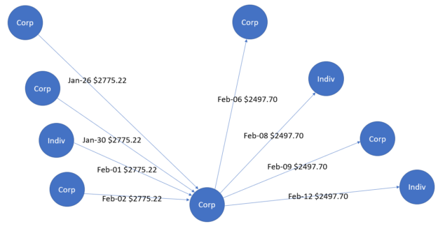
To show the utility of graphs, here’s an example. Mark the businesses and individuals with different titles: businesses are marked as “Corp” and individuals are marked as “Indiv”. The edges are used to represent transactions with associated dates and amounts and the arrows represent the direction of transactions.
There are various expected graph patterns, such as a normal scatter pattern, also known as a dandelion, that happens when an organization pays salaries. Such a pattern occurs on certain dates, salaries are relatively fixed, and the money flow is outbound from a single payer. An anomalous scatter pattern has a sudden burst of transactions that has never been seen previously for involved nodes or bidirectional money flows.
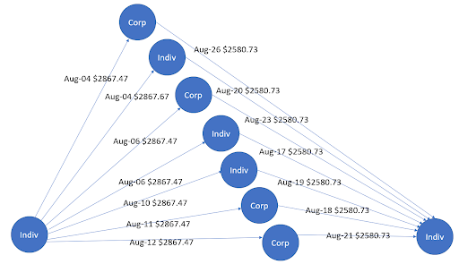
Figure 1 shows a gather-scatter pattern, where money flows initially inbound to the central node in the month of January. These flows are subsequently outbound to other nodes in the month of February. In the world of money-laundering, this gather-scatter pattern is used to hide the distribution of funds from financial institutions. Similarly, Figure 2 shows a scatter-gather pattern that again has a bidirectional flow of money on different dates. In this case, the source and destination of the money are two different central entities.
Based on tabular features as well as graph features, DL-based GAN methods can detect such fraud patterns, with an example based on using Hopsworks on NVIDIA GPUs. Such methods coexist with rule-based techniques to lead to better results, accuracy, and a confusion matrix.
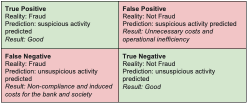
Challenges in modelling fraud as a binary classification problem
Figure 3 shows the confusion matrix of a financial fraud binary classifier. For problems such as money laundering, false negatives should be weighed significantly higher. Use a variant of the F1 score to evaluate models: precision, recall, and fallout should not be weighted equally.
There are other challenges in detecting money laundering patterns:
- Massive class imbalance—Transactions labeled as suspicious may be less than 0.0001% of total historical transactions.
- Non-stationarity—New money-laundering schemes are constantly being invented. To identify new patterns as they appear, techniques must be able to adapt themselves or be easily adapted.
Logical Clocks, developers of the open-source Hopsworks platform, have published as open source a full end-to-end example for detecting fraud:
- A sample raw dataset of financial transactions
- Feature engineering programs to compute complex features such as graph embedding and store them in a feature store
- Notebooks to find good hyperparameters for the GANs
- Distributed training of a GAN using many GPUs.
The code can be reproduced on any Hopsworks cluster, including managed Hopsworks clusters available on AWS, Microsoft Azure, and on-premises installations of Hopsworks with NVIDIA GPUs. Hopsworks clusters can manage up to thousands of GPUs and allocate them to applications on-demand.
NVIDIA GPUs for accelerating financial data science
Identifying fraud and money laundering among large numbers of customer records is a classic financial machine learning (ML) and deep learning (DL) use case. Because it requires many trillion floating point operations (TOPS), applying GPUs accelerates the neural network training process significantly. Many data scientists know that NVIDIA GPUs have been helping in the ML training process for several years.
When the neural network training is complete and the inference phase becomes more important, the recently introduced open-source software NVIDIA Triton Inference Server can help simplify and manage inference acceleration and production model deployment. Triton Server can run as a Docker container, on bare metal, or inside a virtual machine in a virtualized environment. Hopsworks supports serving models on Triton Server using KFServing.
Hopsworks supports ML/DL training using TensorFlow, PyTorch, and Scikit-Learn with additional support for transparent data-parallel training, hyperparameter tuning, and parallel ablation studies on TensorFlow and PyTorch using the Maggy framework. Hopsworks works with multi-GPU, single-node systems as well as clusters of multi-GPU systems. DGX A100 systems are now the universal systems for AI infrastructure for distributed training on the GPU. Each DGX A100 system provides the following configuration:
- 8x NVIDIA 100 Tensor Core GPUs
- 80 GB of GPU memory for a total of 640 GB
- SXM (NVLink) form factor
- Connected with NVIDIA NV Switches
- 5 AI petaFLOPS or 10 petaOPS INT8, respectively
Multi-GPU, multi-node DGX A100 systems constitute superpods on the Hopsworks platform, which can accelerate DL training and inferencing workloads considerably. You can achieve similar configurations on NVIDIA GPUs by working with the NVIDIA Partner Network (NPN) of OEM partners, system integrators, and value-added resellers.
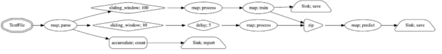
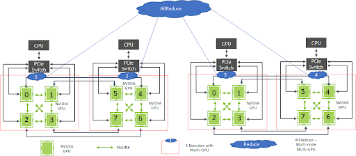
Figure 4 shows the architecture of DL systems using Hopsworks that can leverage data-parallel distributed GPU training using TensorFlow CollectiveAllReduceStrategy. The Maggy framework, supported in Hopsworks, facilitates the ease of development with TensorFlow CollectiveAllReduceStrategy on multi-GPU, multi-node systems, through the transparent management of distribution using Spark. Large clusters additionally benefit from GPU interlinks using NVSwitch. In the future, such an architecture will also be possible using the NVIDIA Rapids.ai framework and Spark on GPUs.
Optimizing distributed training using Hopsworks on NVIDIA-certified multi-GPU, multi-node systems
For inferencing of trained models using other architectures, NVIDIA supports multiple inferencing workloads, concurrent applications, and instances of DL models with the NVIDIA Triton Inferencing Server framework, increasing GPU utilization. Hopsworks clients have used GANs, vision, and other DL models requiring extensive distributed training on the GPU to develop cutting-edge AI systems.
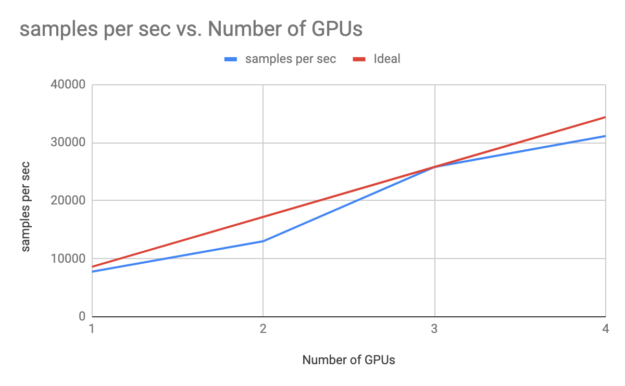
In the following end-to-end money-laundering example from LogicalClocks, a GAN model for anomaly detection was trained on DGX systems using a setup on a multi-GPU, multi-node framework. Training times using such setups can provide almost linear scaling, also known as strong scaling, to accelerate your DL training. Also, inferencing of such models using the Triton Server framework can use the GPUs efficiently.
You can also use other frameworks including RAPIDS.ai, Spark on GPU, and the NVIDIA GRAPH framework CuGraph for accelerating such features on the GPU on the Hopsworks platform.
Get in touch with us
Teamwork is the key to engineering accurate financial fraud and money laundering solutions. Going from rule-based to model-based approaches is a common technology objective. The goal is to reduce the number of falsely classified outcomes that financial institutions may receive when using fraud detection or money laundering models in production. Nowadays, customers expect more accuracy from their financial firms in terms of preventing fraud and limiting false alarms.
For more information and to share your experiences with this important use case and state-of-the-art approach, please leave a comment below.

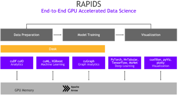
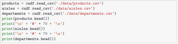
 This tutorial is the seventh installment of introductions to the RAPIDS ecosystem. The series explores and discusses various aspects of RAPIDS that allow its users solve ETL (Extract, Transform, Load) problems, build ML (Machine Learning) and DL (Deep Learning) models, explore expansive graphs, process geospatial, signal, and system log data, or use SQL language via …