Category: Offsites

Posted by Bryan Perozzi, Research Scientist and Qi Zhu, Research Intern, Google Research

Graph Neural Networks (GNNs) are powerful tools for leveraging graph-structured data in machine learning. Graphs are flexible data structures that can model many different kinds of relationships and have been used in diverse applications like traffic prediction, rumor and fake news detection, modeling disease spread, and understanding why molecules smell.

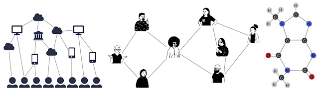
Graphs can model the relationships between many different types of data, including web pages (left), social connections (center), or molecules (right).

As is standard in machine learning (ML), GNNs assume that training samples are selected uniformly at random (i.e., are an independent and identically distributed or “IID” sample). This is easy to do with standard academic datasets, which are specifically created for research analysis and therefore have every node already labeled. However, in many real world scenarios, data comes without labels, and labeling data can be an onerous process involving skilled human raters, which makes it difficult to label all nodes. In addition, biased training data is a common issue because the act of selecting nodes for labeling is usually not IID. For example, sometimes fixed heuristics are used to select a subset of data (which shares some characteristics) for labeling, and other times, human analysts individually choose data items for labeling using complex domain knowledge.

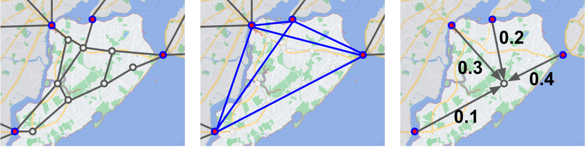
Localized training data is a typical non-IID bias exhibited in graph-structured data. This is shown on the left figure by taking an orange node and expanding to those around it. Instead, an IID training sample of nodes for labeling would be uniformly distributed, as illustrated by the sampling process on the right.

To quantify the amount of bias present in a training set, one can use methods that measure how large the shift is between two different probability distributions, where the size of the shift can be thought of as the amount of bias. As the shift grows in size, machine learning models have more difficulty generalizing from the biased training set. This situation can meaningfully hurt generalizability — on academic datasets, we’ve observed domain shifts causing a performance drop of 15-20% (as measured by the F1 score).

In “Shift-Robust GNNs: Overcoming the Limitations of Localized Graph Training Data”, presented at NeurIPS 2021, we introduce a solution for using GNNs on biased data. Called Shift-Robust GNN (SR-GNN), this approach is designed to account for distributional differences between biased training data and a graph’s true inference distribution. SR-GNN adapts GNN models to the presence of distributional shift between the nodes labeled for training and the rest of the dataset. We illustrate the effectiveness of SR-GNN in a variety of experiments with biased training datasets on common GNN benchmark datasets for semi-supervised learning and show that SR-GNN outperforms other GNN baselines in accuracy, reducing the negative effects of biased training data by 30–40%.

The Impact of Distribution Shifts on Performance
To demonstrate how distribution shift affects GNN performance, we first generate a number of biased training sets for known academic datasets. Then in order to understand the effect, we plot the generalization (test accuracy) versus a measure of distribution shift (the Central Moment Discrepancy¹, CMD). For example, consider the well known PubMed citation dataset, which can be thought of as a graph where the nodes are medical research papers and the edges represent citations between them. When we generate biased training data for PubMed, the plot looks like this:

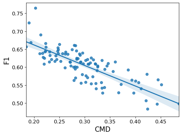
The effect of distribution shift on the PubMed dataset. Performance (F1) is shown on the y-axis vs. the distribution shift, Central Moment Discrepancy (CMD), on the x-axis, for 100 biased training set samples. As the distribution shift increases, the model’s accuracy falls.

Here one can observe a strong negative correlation between the distribution shift in the dataset and the classification accuracy: as CMD increases, the performance (F1) decreases. That is, GNNs can have difficulty generalizing as their training data looks less like the test dataset.

To address this, we propose a shift-robust regularizer (similar in idea to domain-invariant learning) to minimize the distribution shift between training data and an IID sample from unlabeled data. To do this, we measure the domain shift (e.g., via CMD) in real time as the model is training and apply a direct penalty based on this that forces the model to ignore as much of the training bias as possible. This forces the feature encoders that the model learns for the training data to also work effectively for any unlabeled data, which might come from a different distribution.

The figure below shows what this looks like when compared to a traditional GNN model. We still have the same inputs (the node features X, and the Adjacency Matrix A), and the same number of layers. However at the final embedding Z_k from layer (k) of the GNN is compared against embeddings from unlabeled data points to verify that the model is correctly encoding them.

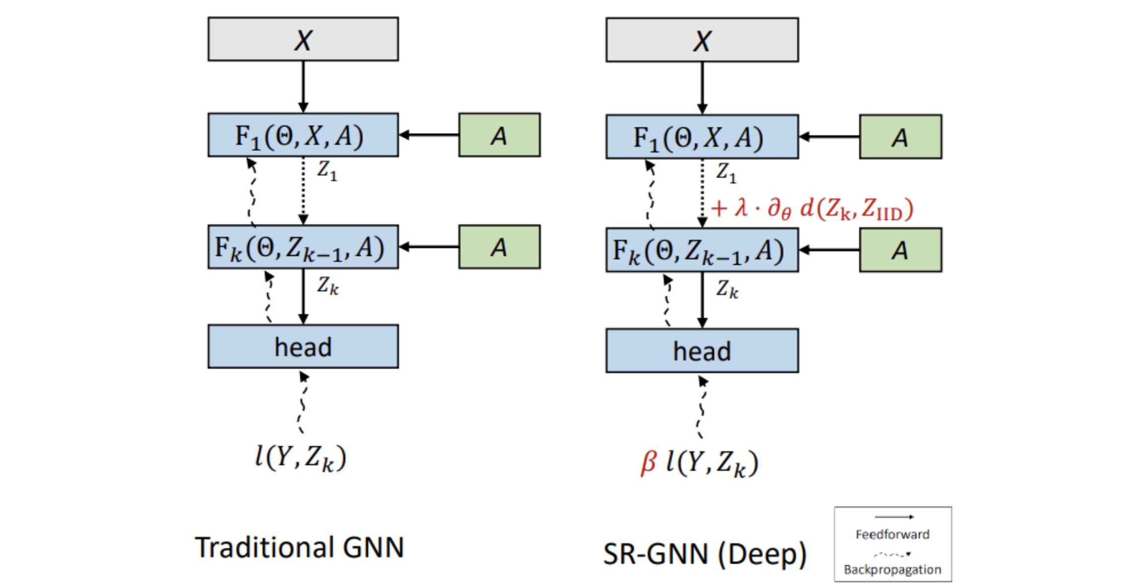
SR-GNN adds two kinds of regularizations to deep GNN models. First, a domain shift regularization (λ term) minimizes the distance between hidden representations of the labeled (Zk) and unlabeled (ZIID) data. Second, the instance weight (β) of the examples can be changed to further approximate the true distribution.

We write this regularization as an additional term in the formula for the model’s loss based on the distance between the training data’s representations and the true data’s distribution (full formulas available in the paper).

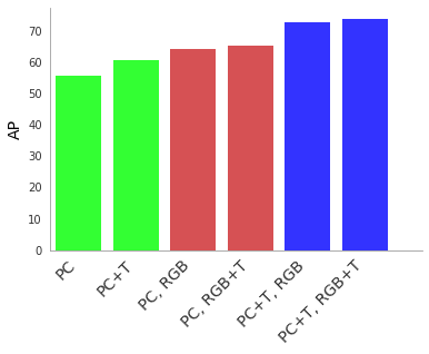
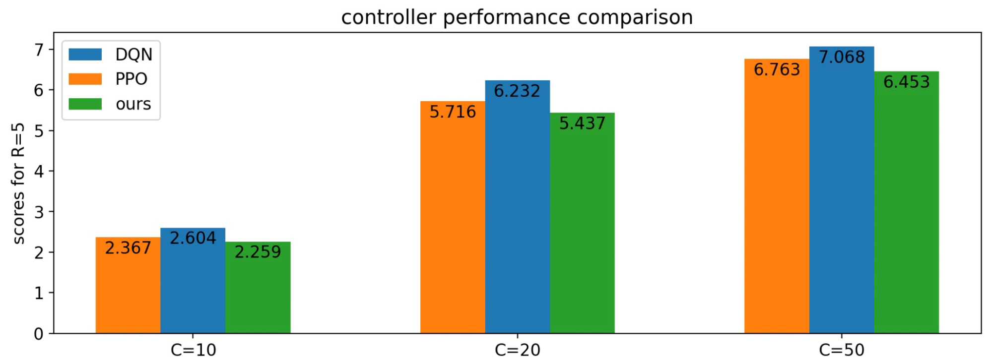
In our experiments, we compare our method and a number of standard graph neural network models, to measure their performance on node classification tasks. We demonstrate that adding the SR-GNN regularization gives a 30–40% percent improvement on classification tasks with biased training data labels.

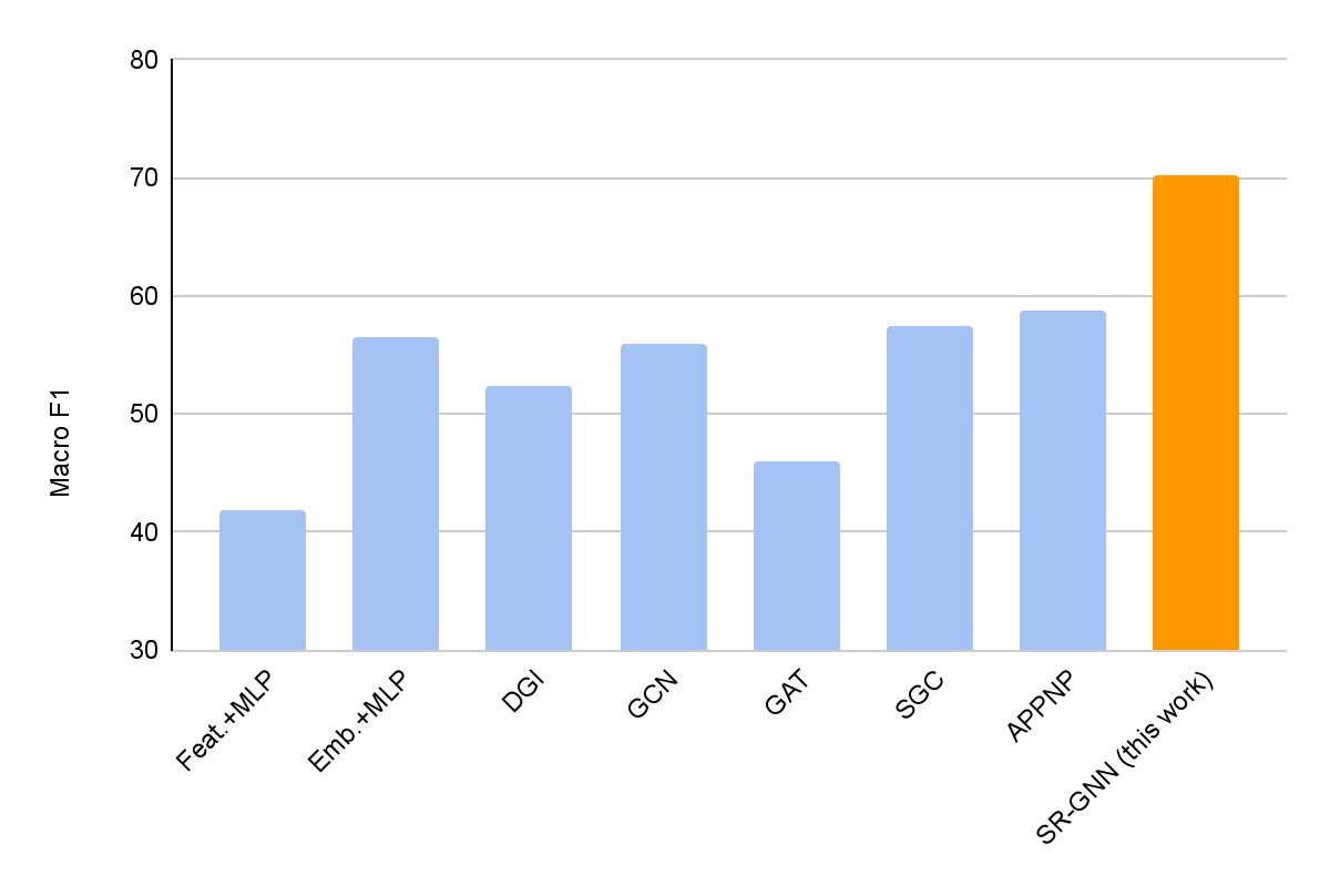
A comparison of SR-GNN using node classification with biased training data on the PubMed dataset. SR-GNN outperforms seven baselines, including DGI, GCN, GAT, SGC and APPNP.

Shift-Robust Regularization for Linear GNNs via Instance Re-weighting
Moreover, it’s worth noting that there’s another class of GNN models (e.g., APPNP, SimpleGCN, etc) that are based on linear operations to speed up their graph convolutions. We also examined how to make these models more reliable in the presence of biased training data. While the same regularization mechanism can not be directly applied due to their different architecture, we can “correct” the training bias by re-weighting the training instances according to their distance from an approximated true distribution. This allows correcting the distribution of the biased training data without passing gradients through the model.

Finally, the two regularizations — for both deep and linear GNNs — can be combined into a generalized regularization for the loss, which combines both domain regularization and instance reweighting (details, including the loss formulas, available in the paper).

Conclusion
Biased training data is common in real world scenarios and can arise due to a variety of reasons, including difficulties of labeling a large amount of data, the various heuristics or inconsistent techniques that are used to choose nodes for labeling, delayed label assignment, and others. We presented a general framework (SR-GNN) that can reduce the influence of biased training data and can be applied to various types of GNNs, including both deeper GNNs and more recent linearized (shallow) versions of these models.

Acknowledgements
Qi Zhu is a PhD Student at UIUC. Thanks to our collaborators Natalia Ponomareva (Google Research) and Jiawei Han (UIUC). Thanks to Tom Small and Anton Tsitsulin for visualizations.

---

¹We note that many measures of distribution shift have been proposed in the literature. Here we use CMD (as it is quick to calculate and generally shows good performance in the domain adaptation literature), but the concept generalizes to any measure of distribution distances/domain shift. ^↩

Posted by Zizhao Zhang and Guanhang Wu, Software Engineers, Google Research, Cloud AI Team

Video recognition is a core task in computer vision with applications from video content analysis to action recognition. However, training models for video recognition often requires untrimmed videos to be manually annotated, which can be prohibitively time consuming. In order to reduce the effort of collecting videos with annotations, learning visual knowledge from videos with weak labels, i.e., where the annotation is auto-generated without manual intervention, has attracted growing research interest, thanks to the large volume of easily accessible video data. Untrimmed videos, for example, are often acquired by querying with keywords for classes that the video recognition model aims to classify. A keyword, which we refer to as a weak label, is then assigned to each untrimmed video obtained.

Although large-scale videos with weak labels are easier to collect, training with unverified weak labels poses another challenge in developing robust models. Recent studies have demonstrated that, in addition to the label noise (e.g., incorrect action labels on untrimmed videos), there is temporal noise due to the lack of accurate temporal action localization — i.e., an untrimmed video may include other non-targeted content or may only show the target action in a small proportion of the video.

Reducing noise effects for large-scale weakly-supervised pre-training is critical but particularly challenging in practice. Recent work indicates that querying short videos (e.g., ~1 minute in length) to obtain more accurate temporal localization of target actions or applying a teacher model to do filtering can yield improved results. However, such data pre-processing methods prevent models from fully utilizing available video data, especially longer videos with richer content.

In “Learning from Weakly-Labeled Web Videos via Exploring Sub-Concepts“, we propose a solution to these issues that uses a simple learning framework to conduct effective pre-training on untrimmed videos. Instead of simply filtering the potential temporal noise, this approach converts such “noisy” data to useful supervision by creating a new set of meaningful “middle ground” pseudo-labels that expand the original weak label space, a novel concept we call Sub-Pseudo Label (SPL). The model is pre-trained on this more “fine-grained” space and then fine-tuned on a target dataset. Our experiments demonstrate that the learned representations are much better than previous approaches. Moreover, SPL has been shown to be effective in improving the action recognition model quality for Google Cloud Video AI, which enables content producers to easily search through massive libraries of their video assets to quickly source content of interest.

Sampled training clips may represent a different visual action (whisking eggs) from the query label of the whole untrimmed video (baking cookies). SPL converts the potential label noise to useful supervision signals by creating a new set of “middle ground” pseudo-classes (i.e., sub-concepts) via extrapolating two related action classes. Enriched supervision is provided for effective model pre-training.

Sub-Pseudo Label (SPL)
SPL is a simple technique that advances the teacher-student training framework, which is known to be effective for self-training and to improve semi-supervised learning. In the teacher-student framework, a teacher model is trained on high-quality labeled data and then assigns pseudo-labels to unlabeled data. The student model trains on both high-quality labeled data and the unlabeled data that has the teacher-predicted labels. While previous methods have proposed a number of ways to improve the pseudo-label quality, SPL takes a novel approach that combines knowledge from both weak labels (i.e., query text used to acquire data) and teacher-predicted labels, which results in better pseudo-labels overall. This method focuses on video recognition where temporal noise is challenging, but it can be extended easily to other domains, like image classification.

The overall pre-training framework for learning from weakly labeled videos via SPLs. Each trimmed video clip is re-labeled using SPL given the teacher-predicted labels and the weak labels used to query the corresponding untrimmed video.

The SPL method is motivated by the observation that within an untrimmed video “noisy” video clips have semantic relations with the target action (i.e., the weak label class), but may also include essential visual components of other actions, such as the teacher model–predicted class. Our approach uses the extrapolated SPLs from weak labels together with the distilled labels to capture the enriched supervision signals, encouraging learning better representations during pre-training that can be used for downstream fine-tuning tasks.

It is straightforward to determine the SPL class for each video clip. We first perform inference on each video clip using the teacher model trained from a target dataset to get a teacher prediction class. Each clip is also labeled by the class (i.e., query text) of the untrimmed source video. A 2-dimensional confusion matrix is used to summarize the alignments between the teacher model inferences and the original weak annotations. Based on this confusion matrix, we conduct label extrapolation between teacher model predictions and weak labels to obtain the raw SPL label space.

Left: The confusion matrix, which is the basis of the raw SPL label space. Middle: The resulting SPL label spaces (16 classes in this example). Right: SPL-B, another SPL version, that reduces the label space by collating agreed and disagreed entries of each row as independent SPL classes, which in this example results in only 8 classes.

Effectiveness of SPL
We evaluate the effectiveness of SPL in comparison to different pre-training methods applied to a 3D ResNet50 model that is fine-tuned on Kinetics-200 (K200). One pre-training approach simply initializes the model using ImageNet. The other pre-training methods use 670k video clips sampled from an internal dataset of 147k videos, collected following standard processes similar to those described for Kinetics-200, that cover a broad range of actions. Weak label training and teacher prediction training use either the weak labels or teacher-predicted labels on the videos, respectively. Agreement filtering uses only the training data for which the weak labels and teacher-predicted labels match. We find that SPL outperforms each of these methods. Though the dataset used to illustrate the SPL approach was constructed for this work, in principle the method we describe applies to any dataset that has weak labels.

Pre-training Method		Top-1		Top-5
ImageNet Initialized		80.6		94.7
Weak Label Train		82.8		95.6
Teacher Prediction Train		81.9		95.0
Agreement Filtering Train		82.9		95.4
SPL		84.3		95.7

We also demonstrate that sampling more video clips from a given number of untrimmed videos can help improve the model performance. With a sufficient number of video clips available, SPL methods consistently outperform weak label pre-training by providing enriched supervision.

As more clips are sampled from 147K videos, the label noise is increased gradually. SPL becomes more and more effective at utilizing the weakly-labeled clips to achieve better pre-training.

We visualize the visual concepts learned from SPL with attention visualization by applying Grad-CAM on the trained model. It is interesting to observe some meaningful “middle ground” concepts that can be learned by SPL.

Examples of attention visualization for SPL classes. Some meaningful “middle ground” concepts can be learned by SPL, such as mixing up the eggs and flour (left) and using the abseiling equipment (right).

Conclusion
We demonstrate that SPLs can provide enriched supervision for pre-training. SPL does not increase training complexity and can be treated as an off-the-shelf technique to integrate with teacher-student–based training frameworks. We believe this is a promising direction for discovering meaningful visual concepts by bridging weak labels and the knowledge distilled from teacher models. SPL has also demonstrated promising generalization to the image recognition domain and we expect future extensions that apply to tasks that have noise in labels. We have successfully applied SPL for Google Cloud Video AI where it has improved the accuracy of the action recognition models, helping users to better understand, search, and monetize their video content library.

Acknowledgements
We gratefully acknowledge the contributions of other co-authors, including Kunpeng Li, Xuehan Xiong, Chen-Yu Lee, Zhichao Lu, Yun Fu, Tomas Pfister. We also thank Debidatta Dwibedi, David A Ross, Chen Sun, Jonathan C. Stroud, and Wei Hua for their valuable comments and help on this work, and Tom Small for figure creation.

Posted by Joel Shor, Staff Software Engineer, Google Research

In recent years, we have seen dramatic improvements on lexical tasks such as automatic speech recognition (ASR). However, machine systems still struggle to understand paralinguistic aspects — such as tone, emotion, whether a speaker is wearing a mask, etc. Understanding these aspects represents one of the remaining difficult problems in machine hearing. In addition, state-of-the-art results often come from ultra-large models trained on private data, making them impractical to run on mobile devices or to release publicly.

In “Universal Paralinguistic Speech Representations Using Self-Supervised Conformers”, to appear in ICASSP 2022, we introduce CAP12— the 12th layer of a 600M parameter model trained on the YT-U training dataset using self-supervision. We demonstrate that the CAP12 model outperforms nearly all previous results in our paralinguistic benchmark, sometimes by large margins, even though previous results are often task-specific. In “TRILLsson: Distilled Universal Paralinguistic Speech Representations”, we introduce the small, performant, publicly-available TRILLsson models and demonstrate how we reduced the size of the high-performing CAP12 model by 6x-100x while maintaining 90-96% of the performance. To create TRILLsson, we apply knowledge distillation on appropriately-sized audio chunks and use different architecture types to train smaller, faster networks that are small enough to run on mobile devices.

1M-Hour Dataset to Train Ultra-Large Self-Supervised Models
We leverage the YT-U training dataset to train the ultra-large, self-supervised CAP12 model. The YT-U dataset is a highly varied, 900M+ hour dataset that contains audio of various topics, background conditions, and speaker acoustic properties.

Video categories by length (outer) and number (inner), demonstrating the variety in the YT-U dataset (figure from BigSSL)

We then modify a Wav2Vec 2.0 self-supervised training paradigm, which can solve tasks using raw data without labels, and combine it with ultra-large Conformer models. Because self-training doesn’t require labels, we can take full advantage of YT-U by scaling up our models to some of the largest model sizes ever trained, including 600M, 1B, and 8B parameters.

NOSS: A Benchmark for Paralinguistic Tasks
We demonstrate that an intermediate representation of one of the previous models contains a state-of-the-art representation for paralinguistic speech. We call the 600M parameter Conformer model without relative attention Conformer Applied to Paralinguistics (CAP). We exhaustively search through all intermediate representations of six ultra-large models and find that layer 12 (CAP12) outperforms previous representations by significant margins.

To measure the quality of the roughly 300 candidate paralinguistic speech representations, we evaluate on an expanded version of the NOn-Semantic Speech (NOSS) benchmark, which is a collection of well-studied paralinguistic speech tasks, such as speech emotion recognition, language identification, and speaker identification. These tasks focus on paralinguistics aspects of speech, which require evaluating speech features on the order of 1 second or longer, rather than lexical features, which require 100ms or shorter. We then add to the benchmark a mask-wearing task introduced at Interspeech 2020, a fake speech detection task (ASVSpoof 2019), a task to detect the level of dysarthria from project Euphonia, and an additional speech emotion recognition task (IEMOCAP). By expanding the benchmark and increasing the diversity of the tasks, we empirically demonstrate that CAP12 is even more generally useful than previous representations.

Simple linear models on time-averaged CAP12 representations even outperform complex, task-specific models on five out of eight paralinguistic tasks. This is surprising because comparable models sometimes use additional modalities (e.g., vision and speech, or text and speech) as well. Furthermore, CAP12 is exceptionally good at emotion recognition tasks. CAP12 embeddings also outperform all other embeddings on all other tasks with only a single exception: for one embedding from a supervised network on the dysarthria detection task.

Model	Voxceleb†	Voxforge	Speech Commands	ASVSpoof2019∗∗	Euphonia#	CREMA-D	IEMOCAP
Prev SoTA	–	95.4	97.9	5.11	45.9	74.0∗	67.6+
TRILL	12.6	84.5	77.6	74.6	48.1	65.7	54.3
ASR Embedding	5.2	98.9	96.1	11.2	54.5	71.8	65.4
Wav2Vec2 layer 6††	17.9	98.5	95.0	6.7	48.2	77.4	65.8
CAP12	51.0	99.7	97.0	2.5	51.5	88.2	75.0

Test performance on the NOSS Benchmark and extended tasks. “Prev SoTA” indicates the previous best performing state-of-the-art model, which has arbitrary complexity, but all other rows are linear models on time-averaged input. † Filtered according to YouTube’s privacy guidelines. ∗∗ Uses equal error rate [20]. # The only non-public dataset. We exclude it from aggregate scores. ∗ Audio and visual features used in previous state-of-the-art models. + The previous state-of-the-art model performed cross-validation. For our evaluation, we hold out two specific speakers as a test. †† Wav2Vec 2.0 model from HuggingFace. Best overall layer was layer 6.

TRILLsson: Small, High Quality, Publicly Available Models
Similar to FRILL, our next step was to make an on-device, publicly available version of CAP12. This involved using knowledge distillation to train smaller, faster, mobile-friendly architectures. We experimented with EfficientNet, Audio Spectrogram Transformer (AST), and ResNet. These model types are very different, and cover both fixed-length and arbitrary-length inputs. EfficientNet comes from a neural architecture search over vision models to find simultaneously performant and efficient model structures. AST models are transformers adapted to audio inputs. ResNet is a standard architecture that has shown good performance across many different models.

We trained models that performed on average 90-96% as well as CAP12, despite being 1%-15% the size and trained using only 6% the data. Interestingly, we found that different architecture types performed better at different sizes. ResNet models performed best at the low end, EfficientNet in the middle, and AST models at the larger end.

Aggregate embedding performance vs. model size for various student model architectures and sizes. We demonstrate that ResNet architectures perform best for small sizes, EfficientNetV2 performs best in the midsize model range, up to the largest model size tested, after which the larger AST models are best.

We perform knowledge distillation with the goal of matching a student, with a fixed-size input, to the output of a teacher, with a variable-size input, for which there are two methods of generating student targets: global matching and local matching. Global matching produces distillation targets by generating CAP12 embeddings for an entire audio clip, and then requires that a student match the target from just a small segment of audio (e.g., 2 seconds). Local matching requires that the student network match the average CAP12 embedding just over the smaller portion of the audio that the student sees. In our work, we focused on local matching.

Two types of generating distillation targets for sequences. Left: Global matching uses the average CAP12 embedding over the whole clip for the target for each local chunk. Right: Local matching uses CAP12 embeddings averaged just over local clips as the distillation target.

Observation of Bimodality and Future Directions
Paralinguistic information shows an unexpected bimodal distribution. For the CAP model that operates on 500 ms input segments, and two of the full-input Conformer models, intermediate representations gradually increase in paralinguistic information, then decrease, then increase again, and finally lose this information towards the output layer. Surprisingly, this pattern is also seen when exploring the intermediate representations of networks trained on retinal images.

500 ms inputs to CAP show a relatively pronounced bimodal distribution of paralinguistic information across layers.

Two of the conformer models with full inputs show a bimodal distribution of paralinguistic information across layers.

We hope that smaller, faster models for paralinguistic speech unlock new applications in speech recognition, text-to-speech generation, and understanding user intent. We also expect that smaller models will be more easily interpretable, which will allow researchers to understand what aspects of speech are important for paralinguistics. Finally, we hope that our open-sourced speech representations are used by the community to improve paralinguistic speech tasks and user understanding in private or small datasets.

Acknowledgements
I’d like to thank my co-authors Aren Jansen, Wei Han, Daniel Park, Yu Zhang, and Subhashini Venugopalan for their hard work and creativity on this project. I’d also like to thank the members of the large collaboration for the BigSSL work, without which these projects would not be possible. The team includes James Qin, Anmol Gulati, Yuanzhong Xu, Yanping Huang, Shibo Wang, Zongwei Zhou, Bo Li, Min Ma, William Chan, Jiahui Yu, Yongqiang Wang, Liangliang Cao, Khe Chai Sim, Bhuvana Ramabhadran, Tara N. Sainath, Françoise Beaufays, Zhifeng Chen, Quoc V. Le, Chung-Cheng Chiu, Ruoming Pang, and Yonghui Wu.

Posted by Maxwell Bileschi, Staff Software Engineer and Lucy Colwell, Research Scientist, Google Research, Brain Team

Proteins are essential molecules found in all living things. They play a central role in our bodies’ structure and function, and they are also featured in many products that we encounter every day, from medications to household items like laundry detergent. Each protein is a chain of amino acid building blocks, and just as an image may include multiple objects, like a dog and a cat, a protein may also have multiple components, which are called protein domains. Understanding the relationship between a protein’s amino acid sequence — for example, its domains — and its structure or function are long-standing challenges with far-reaching scientific implications.

An example of a protein with known structure, TrpCF from E. coli, for which areas used by a model to predict function are highlighted (green). This protein produces tryptophan, which is an essential part of a person’s diet.

<!–

An example of a protein with known structure, TrpCF from E. coli, for which areas used by a model to predict function are highlighted (green). This protein produces tryptophan, which is an essential part of a person’s diet.

–>

Many are familiar with recent advances in computationally predicting protein structure from amino acid sequences, as seen with DeepMind’s AlphaFold. Similarly, the scientific community has a long history of using computational tools to infer protein function directly from sequences. For example, the widely-used protein family database Pfam contains numerous highly-detailed computational annotations that describe a protein domain’s function, e.g., the globin and trypsin families. While existing approaches have been successful at predicting the function of hundreds of millions of proteins, there are still many more with unknown functions — for example, at least one-third of microbial proteins are not reliably annotated. As the volume and diversity of protein sequences in public databases continue to increase rapidly, the challenge of accurately predicting function for highly divergent sequences becomes increasingly pressing.

In “Using Deep Learning to Annotate the Protein Universe”, published in Nature Biotechnology, we describe a machine learning (ML) technique to reliably predict the function of proteins. This approach, which we call ProtENN, has enabled us to add about 6.8 million entries to Pfam’s well-known and trusted set of protein function annotations, about equivalent to the sum of progress over the last decade, which we are releasing as Pfam-N. To encourage further research in this direction, we are releasing the ProtENN model and a distill-like interactive article where researchers can experiment with our techniques. This interactive tool allows the user to enter a sequence and get results for a predicted protein function in real time, in the browser, with no setup required. In this post, we’ll give an overview of this achievement and how we’re making progress toward revealing more of the protein universe.

The Pfam database is a large collection of protein families and their sequences. Our ML model ProtENN helped annotate 6.8 million more protein regions in the database.

Protein Function Prediction as a Classification Problem
In computer vision, it’s common to first train a model for image classification tasks, like CIFAR-100, before extending it to more specialized tasks, like object detection and localization. Similarly, we develop a protein domain classification model as a first step towards future models for classification of entire protein sequences. We frame the problem as a multi-class classification task in which we predict a single label out of 17,929 classes — all classes contained in the Pfam database — given a protein domain’s sequence of amino acids.

Models that Link Sequence to Function
While there are a number of models currently available for protein domain classification, one drawback of the current state-of-the-art methods is that they are based on the alignment of linear sequences and don’t consider interactions between amino acids in different parts of protein sequences. But proteins don’t just stay as a line of amino acids, they fold in on themselves such that nonadjacent amino acids have strong effects on each other.

Aligning a new query sequence to one or more sequences with known function is a key step of current state-of-the-art methods. This reliance on sequences with known function makes it challenging to predict a new sequence’s function if it is highly dissimilar to any sequence with known function. Furthermore, alignment-based methods are computationally intensive, and applying them to large datasets, such as the metagenomic database MGnify, which contains >1 billion protein sequences, can be cost prohibitive.

To address these challenges, we propose to use dilated convolutional neural networks (CNNs), which should be well-suited to modeling non-local pairwise amino-acid interactions and can be run on modern ML hardware like GPUs. We train 1-dimensional CNNs to predict the classification of protein sequences, which we call ProtCNN, as well as an ensemble of independently trained ProtCNN models, which we call ProtENN. Our goal for using this approach is to add knowledge to the scientific literature by developing a reliable ML approach that complements traditional alignment-based methods. To demonstrate this, we developed a method to accurately measure our method’s accuracy.

Evaluation with Evolution in Mind
Similar to well-known classification problems in other fields, the challenge in protein function prediction is less in developing a completely new model for the task, and more in creating fair training and test sets to ensure that the models will make accurate predictions for unseen data. Because proteins have evolved from shared common ancestors, different proteins often share a substantial fraction of their amino acid sequence. Without proper care, the test set could be dominated by samples that are highly similar to the training data, which could lead to the models performing well by simply “memorizing” the training data, rather than learning to generalize more broadly from it.

We create a test set that requires ProtENN to generalize well on data far from its training set.

<!–

We create a test set that requires ProtENN to generalize well on data far from its training set.

–>

To guard against this, it is essential to evaluate model performance using multiple separate setups. For each evaluation, we stratify model accuracy as a function of similarity between each held-out test sequence and the nearest sequence in the train set.

The first evaluation includes a clustered split training and test set, consistent with prior literature. Here, protein sequence samples are clustered by sequence similarity, and entire clusters are placed into either the train or test sets. As a result, every test example is at least 75% different from every training example. Strong performance on this task demonstrates that a model can generalize to make accurate predictions for out-of-distribution data.

For the second evaluation, we use a randomly split training and test set, where we stratify examples based on an estimate of how difficult they will be to classify. These measures of difficulty include: (1) the similarity between a test example and the nearest training example, and (2) the number of training examples from the true class (it is much more difficult to accurately predict function given just a handful of training examples).

To place our work in context, we evaluate the performance of the most widely used baseline models and evaluation setups, with the following baseline models in particular: (1) BLAST, a nearest-neighbor method that uses sequence alignment to measure distance and infer function, and (2) profile hidden Markov models (TPHMM and phmmer). For each of these, we include the stratification of model performance based on sequence alignment similarity mentioned above. We compared these baselines against ProtCNN and the ensemble of CNNs, ProtENN.

We measure each model’s ability to generalize, from the hardest examples (left) to the easiest (right).

Reproducible and Interpretable Results
We also worked with the Pfam team to test whether our methodological proof of concept could be used to label real-world sequences. We demonstrated that ProtENN learns complementary information to alignment-based methods, and created an ensemble of the two approaches to label more sequences than either method could by itself. We publicly released the results of this effort, Pfam-N, a set of 6.8 million new protein sequence annotations.

After seeing the success of these methods and classification tasks, we inspected these networks to understand whether the embeddings were generally useful. We built a tool that enables users to explore the relation between the model predictions, embeddings, and input sequences, which we have made available through our interactive manuscript, and we found that similar sequences were clustered together in embedding space. Furthermore, the network architecture that we selected, a dilated CNN, allows us to employ previously-discovered interpretability methods like class activation mapping (CAM) and sufficient input subsets (SIS) to identify the sub-sequences responsible for the neural network predictions. With this approach, we find that our network generally focuses on the relevant elements of a sequence to predict its function.

Conclusion and Future Work
We’re excited about the progress we’ve seen by applying ML to the understanding of protein structure and function over the last few years, which has been reflected in contributions from the broader research community, from AlphaFold and CAFA to the multitude of workshops and research presentations devoted to this topic at conferences. As we look to build on this work, we think that continuing to collaborate with scientists across the field who’ve shared their expertise and data, combined with advances in ML will help us further reveal the protein universe.

Acknowledgments
We’d like to thank all of the co-authors of the manuscripts, Maysam Moussalem, Jamie Smith, Eli Bixby, Babak Alipanahi, Shanqing Cai, Cory McLean, Abhinay Ramparasad, Steven Kearnes, Zack Nado, and Tom Small.

Posted by Bowen Zhang, Student Researcher and Jiahui Yu, Senior Research Scientist, Google Research, Brain Team

Action recognition has become a major focus area for the research community because many applications can benefit from improved modeling, such as video retrieval, video captioning, video question-answering, etc. Transformer-based approaches have recently demonstrated state-of-the-art performance on several benchmarks. While Transformer models require data to learn better visual priors compared to ConvNets, action recognition datasets are relatively small in scale. Large Transformer models are typically first trained on image datasets and later fine-tuned on a target action recognition dataset.

While the current pre-training and fine-tuning action recognition paradigm is straightforward and manifests strong empirical results, it may be overly restrictive for building general-purpose action-recognition models. Compared to a dataset like ImageNet that covers a large range of object recognition classes, action recognition datasets like Kinetics and Something-Something-v2 (SSv2) pertain to limited topics. For example, Kinetics include object-centric actions like “cliff diving” and “ice climbing’ while SSv2 contains object-agnostic activities like ’pretending to put something onto something else.’ As a result, we observed poor performance adapting an action recognition model that has been fine-tuned on one dataset to another disparate dataset.

Differences in objects and video backgrounds among datasets further exacerbate learning a general-purpose action recognition classification model. Despite the fact that video datasets may be increasing in size, prior work suggests significant data augmentation and regularization is necessary to achieve strong performance. This latter finding may indicate the model quickly overfits on the target dataset, and as a result, hinders its capacity to generalize to other action recognition tasks.

In “Co-training Transformer with Videos and Images Improves Action Recognition”, we propose a training strategy, named CoVeR, that leverages both image and video data to jointly learn a single general-purpose action recognition model. Our approach is buttressed by two main findings. First, disparate video datasets cover a diverse set of activities, and training them together in a single model could lead to a model that excels at a wide range of activities. Second, video is a perfect source for learning motion information, while images are great for exploiting structural appearance. Leveraging a diverse distribution of image examples may be beneficial in building robust spatial representations in video models. Concretely, CoVeR first pre-trains the model on an image dataset, and during fine-tuning, it simultaneously trains a single model on multiple video and image datasets to build robust spatial and temporal representations for a general-purpose video understanding model.

Architecture and Training Strategy
We applied the CoVeR approach to the recently proposed spatial-temporal video transformer, called TimeSFormer, that contains 24 layers of transformer blocks. Each block contains one temporal attention, one spatial attention, and one multilayer perceptron (MLP) layer. To learn from multiple video and image datasets, we adopt a multi-task learning paradigm and equip the action recognition model with multiple classification heads. We pre-train all non-temporal parameters on the large-scale JFT dataset. During fine-tuning, a batch of videos and images are sampled from multiple video and image datasets. The sampling rate is proportional to the size of the datasets. Each sample within the batch is processed by the TimeSFormer and then distributed to the corresponding classifier to get the predictions.

Compared with the standard training strategy, CoVeR has two advantages. First, as the model is directly trained on multiple datasets, the learned video representations are more general and can be directly evaluated on those datasets without additional fine-tuning. Second, Transformer-based models may easily overfit to a smaller video distribution, thus degrading the generalization of the learned representations. Training on multiple datasets mitigates this challenge by reducing the risk of overfitting.

CoVeR adopts a multi-task learning strategy trained on multiple datasets, each with their own classifier.

Benchmark Results
We evaluate the CoVeR approach to train on Kinetics-400 (K400), Kinetics-600 (K600), Kinetics-700 (K700), SomethingSomething-V2 (SSv2), and Moments-in-Time (MiT) datasets. Compared with other approaches — such as TimeSFormer, Video SwinTransformer, TokenLearner, ViViT, MoViNet, VATT, VidTr, and OmniSource — CoVeR established the new state-of-the-art on multiple datasets (shown below). Unlike previous approaches that train a dedicated model for one single dataset, a model trained by CoVeR can be directly applied to multiple datasets without further fine-tuning.

Model	Pretrain	Finetune	K400 Accuracy
VATT	AudioSet+Videos	K400	82.1
Omnisource	IG-Kinetics-65M	K400	83.6
ViViT	JFT-300M	K400	85.4
Video SwinTrans	ImageNet21K+external	K400	86.8
CoVeR	JFT-3B	K400+SSv2+MiT+ImNet	87.2

Accuracy comparison on Kinetics-400 (K400) dataset.

Model	Pretrain	Finetune	SSv2 Accuracy
TimeSFormer	ImageNet21k	SSv2	62.4
VidTr	ImageNet21k	SSv2	63.0
ViViT	ImageNet21k	SSv2	65.9
Video SwinTrans	ImageNet21K+external	SSv2	69.6
CoVeR	JFT-3B	K400+SSv2+MiT+ImNet	70.9

Accuracy comparison on SomethingSomething-V2 (SSv2) dataset.

Model	Pretrain	Finetune	MiT Accuracy
ViViT	ImageNet21k	MiT	38.5
VidTr	ImageNet21k	SSv2	41.1
CoVeR	JFT-3B	K400+SSv2+MiT+ImNet	46.1

Accuracy comparison on Moments-in-Time (MiT) dataset.

Transfer Learning
We use transfer learning to further verify the video action recognition performance and compare with co-training on multiple datasets, results are summarized below. Specifically, we train on the source datasets, then fine-tune and evaluate on the target dataset.

We first consider K400 as the target dataset. CoVeR co-trained on SSv2 and MiT improves the top-1 accuracy on K400→K400 (where the model is trained on K400 and then fine-tuned on K400) by 1.3%, SSv2→K400 by 1.7%, and MiT→K400 by 0.4%. Similarly, we observe that by transferring to SSv2, CoVeR achieves 2%, 1.8%, and 1.1% improvement over SSv2→SSv2, K400→SSv2, and MiT→SSv2, respectively. The 1.2% and 2% performance improvement on K400 and SSv2 indicates that CoVeR co-trained on multiple datasets could learn better visual representations than the standard training paradigm, which is useful for downstream tasks.

Comparison of transfer learning the representation learned by CoVeR and standard training paradigm. A→B means the model is trained on dataset A and then fine-tuned on dataset B.

Conclusion
In this work, we present CoVeR, a training paradigm that jointly learns action recognition and object recognition tasks in a single model for the purpose of constructing a general-purpose action recognition framework. Our analysis indicates that it may be beneficial to integrate many video datasets into one multi-task learning paradigm. We highlight the importance of continuing to learn on image data during fine-tuning to maintain robust spatial representations. Our empirical findings suggest CoVeR can learn a single general-purpose video understanding model which achieves impressive performance across many action recognition datasets without an additional stage of fine-tuning on each downstream application.

Acknowledgements
We would like to thank Christopher Fifty, Wei Han, Andrew M. Dai, Ruoming Pang, and Fei Sha for preparation of the CoVeR paper, Yue Zhao, Hexiang Hu, Zirui Wang, Zitian Chen, Qingqing Huang, Claire Cui and Yonghui Wu for helpful discussions and feedbacks, and others on the Brain Team for support throughout this project.

Posted by Brendan McMahan and Abhradeep Thakurta, Research Scientists, Google Research

In 2017, Google introduced federated learning (FL), an approach that enables mobile devices to collaboratively train machine learning (ML) models while keeping the raw training data on each user’s device, decoupling the ability to do ML from the need to store the data in the cloud. Since its introduction, Google has continued to actively engage in FL research and deployed FL to power many features in Gboard, including next word prediction, emoji suggestion and out-of-vocabulary word discovery. Federated learning is improving the “Hey Google” detection models in Assistant, suggesting replies in Google Messages, predicting text selections, and more.

While FL allows ML without raw data collection, differential privacy (DP) provides a quantifiable measure of data anonymization, and when applied to ML can address concerns about models memorizing sensitive user data. This too has been a top research priority, and has yielded one of the first production uses of DP for analytics with RAPPOR in 2014, our open-source DP library, Pipeline DP, and TensorFlow Privacy.

Through a multi-year, multi-team effort spanning fundamental research and product integration, today we are excited to announce that we have deployed a production ML model using federated learning with a rigorous differential privacy guarantee. For this proof-of-concept deployment, we utilized the DP-FTRL algorithm to train a recurrent neural network to power next-word-prediction for Spanish-language Gboard users. To our knowledge, this is the first production neural network trained directly on user data announced with a formal DP guarantee (technically ρ=0.81 zero-Concentrated-Differential-Privacy, zCDP, discussed in detail below). Further, the federated approach offers complimentary data minimization advantages, and the DP guarantee protects all of the data on each device, not just individual training examples.

Data Minimization and Anonymization in Federated Learning
Along with fundamentals like transparency and consent, the privacy principles of data minimization and anonymization are important in ML applications that involve sensitive data.

Federated learning systems structurally incorporate the principle of data minimization. FL only transmits minimal updates for a specific model training task (focused collection), limits access to data at all stages, processes individuals’ data as early as possible (early aggregation), and discards both collected and processed data as soon as possible (minimal retention).

Another principle that is important for models trained on user data is anonymization, meaning that the final model should not memorize information unique to a particular individual’s data, e.g., phone numbers, addresses, credit card numbers. However, FL on its own does not directly tackle this problem.

The mathematical concept of DP allows one to formally quantify this principle of anonymization. Differentially private training algorithms add random noise during training to produce a probability distribution over output models, and ensure that this distribution doesn’t change too much given a small change to the training data; ρ-zCDP quantifies how much the distribution could possibly change. We call this example-level DP when adding or removing a single training example changes the output distribution on models in a provably minimal way.

Showing that deep learning with example-level differential privacy was even possible in the simpler setting of centralized training was a major step forward in 2016. Achieved by the DP-SGD algorithm, the key was amplifying the privacy guarantee by leveraging the randomness in sampling training examples (“amplification-via-sampling”).

However, when users can contribute multiple examples to the training dataset, example-level DP is not necessarily strong enough to ensure the users’ data isn’t memorized. Instead, we have designed algorithms for user-level DP, which requires that the output distribution of models doesn’t change even if we add/remove all of the training examples from any one user (or all the examples from any one device in our application). Fortunately, because FL summarizes all of a user’s training data as a single model update, federated algorithms are well-suited to offering user-level DP guarantees.

Both limiting the contributions from one user and adding noise can come at the expense of model accuracy, however, so maintaining model quality while also providing strong DP guarantees is a key research focus.

The Challenging Path to Federated Learning with Differential Privacy
In 2018, we introduced the DP-FedAvg algorithm, which extended the DP-SGD approach to the federated setting with user-level DP guarantees, and in 2020 we deployed this algorithm to mobile devices for the first time. This approach ensures the training mechanism is not too sensitive to any one user’s data, and empirical privacy auditing techniques rule out some forms of memorization.

However, the amplification-via-samping argument is essential to providing a strong DP guarantee for DP-FedAvg, but in a real-world cross-device FL system ensuring devices are subsampled precisely and uniformly at random from a large population would be complex and hard to verify. One challenge is that devices choose when to connect (or “check in”) based on many external factors (e.g., requiring the device is idle, on unmetered WiFi, and charging), and the number of available devices can vary substantially.

Achieving a formal privacy guarantee requires a protocol that does all of the following:

• Makes progress on training even as the set of devices available varies significantly with time.
• Maintains privacy guarantees even in the face of unexpected or arbitrary changes in device availability.
• For efficiency, allows client devices to locally decide whether they will check in to the server in order to participate in training, independent of other devices.

Initial work on privacy amplification via random check-ins highlighted these challenges and introduced a feasible protocol, but it would have required complex changes to our production infrastructure to deploy. Further, as with the amplification-via-sampling analysis of DP-SGD, the privacy amplification possible with random check-ins depends on a large number of devices being available. For example, if only 1000 devices are available for training, and participation of at least 1000 devices is needed in each training step, that requires either 1) including all devices currently available and paying a large privacy cost since there is no randomness in the selection, or 2) pausing the protocol and not making progress until more devices are available.

Achieving Provable Differential Privacy for Federated Learning with DP-FTRL
To address this challenge, the DP-FTRL algorithm is built on two key observations: 1) the convergence of gradient-descent-style algorithms depends primarily not on the accuracy of individual gradients, but the accuracy of cumulative sums of gradients; and 2) we can provide accurate estimates of cumulative sums with a strong DP guarantee by utilizing negatively correlated noise, added by the aggregating server: essentially, adding noise to one gradient and subtracting that same noise from a later gradient. DP-FTRL accomplishes this efficiently using the Tree Aggregation algorithm [1, 2].

The graphic below illustrates how estimating cumulative sums rather than individual gradients can help. We look at how the noise introduced by DP-FTRL and DP-SGD influence model training, compared to the true gradients (without added noise; in black) which step one unit to the right on each iteration. The individual DP-FTRL gradient estimates (blue), based on cumulative sums, have larger mean-squared-error than the individually-noised DP-SGD estimates (orange), but because the DP-FTRL noise is negatively correlated, some of it cancels out from step to step, and the overall learning trajectory stays closer to the true gradient descent steps.

To provide a strong privacy guarantee, we limit the number of times a user contributes an update. Fortunately, sampling-without-replacement is relatively easy to implement in production FL infrastructure: each device can remember locally which models it has contributed to in the past, and choose to not connect to the server for any later rounds for those models.

Production Training Details and Formal DP Statements
For the production DP-FTRL deployment introduced above, each eligible device maintains a local training cache consisting of user keyboard input, and when participating computes an update to the model which makes it more likely to suggest the next word the user actually typed, based on what has been typed so far. We ran DP-FTRL on this data to train a recurrent neural network with ~1.3M parameters. Training ran for 2000 rounds over six days, with 6500 devices participating per round. To allow for the DP guarantee, devices participated in training at most once every 24 hours. Model quality improved over the previous DP-FedAvg trained model, which offered empirically-tested privacy advantages over non-DP models, but lacked a meaningful formal DP guarantee.

The training mechanism we used is available in open-source in TensorFlow Federated and TensorFlow Privacy, and with the parameters used in our production deployment it provides a meaningfully strong privacy guarantee. Our analysis gives ρ=0.81 zCDP at the user level (treating all the data on each device as a different user), where smaller numbers correspond to better privacy in a mathematically precise way. As a comparison, this is stronger than the ρ=2.63 zCDP guarantee chosen by the 2020 US Census.

Next Steps
While we have reached the milestone of deploying a production FL model using a mechanism that provides a meaningfully small zCDP, our research journey continues. We are still far from being able to say this approach is possible (let alone practical) for most ML models or product applications, and other approaches to private ML exist. For example, membership inference tests and other empirical privacy auditing techniques can provide complimentary safeguards against leakage of users’ data. Most importantly, we see training models with user-level DP with even a very large zCDP as a substantial step forward, because it requires training with a DP mechanism that bounds the sensitivity of the model to any one user’s data. Further, it smooths the road to later training models with improved privacy guarantees as better algorithms or more data become available. We are excited to continue the journey toward maximizing the value that ML can deliver while minimizing potential privacy costs to those who contribute training data.

Acknowledgements
The authors would like to thank Alex Ingerman and Om Thakkar for significant impact on the blog post itself, as well as the teams at Google that helped develop these ideas and bring them to practice:

• Core research team: Galen Andrew, Borja Balle, Peter Kairouz, Daniel Ramage, Shuang Song, Thomas Steinke, Andreas Terzis, Om Thakkar, Zheng Xu
• FL infrastructure team: Katharine Daly, Stefan Dierauf, Hubert Eichner, Igor Pisarev, Timon Van Overveldt, Chunxiang Zheng
• Gboard team: Angana Ghosh, Xu Liu, Yuanbo Zhang
• Speech team: Françoise Beaufays, Mingqing Chen, Rajiv Mathews, Vidush Mukund, Igor Pisarev, Swaroop Ramaswamy, Dan Zivkovic

Posted by Abhishek Kumar and Ehsan Amid, Research Scientists, Google Research, Brain Team

Over the past several years, deep neural networks (DNNs) have been quite successful in driving impressive performance gains in several real-world applications, from image recognition to genomics. However, modern DNNs often have far more trainable model parameters than the number of training examples and the resulting overparameterized networks can easily overfit to noisy or corrupted labels (i.e., examples that are assigned a wrong class label). As a consequence, training with noisy labels often leads to degradation in accuracy of the trained model on clean test data. Unfortunately, noisy labels can appear in several real-world scenarios due to multiple factors, such as errors and inconsistencies in manual annotation and the use of inherently noisy label sources (e.g., the internet or automated labels from an existing system).

Earlier work has shown that representations learned by pre-training large models with noisy data can be useful for prediction when used in a linear classifier trained with clean data. In principle, it is possible to directly train machine learning (ML) models on noisy data without resorting to this two-stage approach. To be successful, such alternative methods should have the following properties: (i) they should fit easily into standard training pipelines with little computational or memory overhead; (ii) they should be applicable in “streaming” settings where new data is continuously added during training; and (iii) they should not require data with clean labels.

In “Constrained Instance and Class Reweighting for Robust Learning under Label Noise”, we propose a novel and principled method, named Constrained Instance reWeighting (CIW), with these properties that works by dynamically assigning importance weights both to individual instances and to class labels in a mini-batch, with the goal of reducing the effect of potentially noisy examples. We formulate a family of constrained optimization problems that yield simple solutions for these importance weights. These optimization problems are solved per mini-batch, which avoids the need to store and update the importance weights over the full dataset. This optimization framework also provides a theoretical perspective for existing label smoothing heuristics that address label noise, such as label bootstrapping. We evaluate the method with varying amounts of synthetic noise on the standard CIFAR-10 and CIFAR-100 benchmarks and observe considerable performance gains over several existing methods.

Method
Training ML models involves minimizing a loss function that indicates how well the current parameters fit to the given training data. In each training step, this loss is approximately calculated as a (weighted) sum of the losses of individual instances in the mini-batch of data on which it is operating. In standard training, each instance is treated equally for the purpose of updating the model parameters, which corresponds to assigning uniform (i.e., equal) weights across the mini-batch.

However, empirical observations made in earlier works reveal that noisy or mislabeled instances tend to have higher loss values than those that are clean, particularly during early to mid-stages of training. Thus, assigning uniform importance weights to all instances means that due to their higher loss values, the noisy instances can potentially dominate the clean instances and degrade the accuracy on clean test data.

Motivated by these observations, we propose a family of constrained optimization problems that solve this problem by assigning importance weights to individual instances in the dataset to reduce the effect of those that are likely to be noisy. This approach provides control over how much the weights deviate from uniform, as quantified by a divergence measure. It turns out that for several types of divergence measures, one can obtain simple formulae for the instance weights. The final loss is computed as the weighted sum of individual instance losses, which is used for updating the model parameters. We call this the Constrained Instance reWeighting (CIW) method. This method allows for controlling the smoothness or peakiness of the weights through the choice of divergence and a corresponding hyperparameter.

Schematic of the proposed Constrained Instance reWeighting (CIW) method.

Illustration with Decision Boundary on a 2D Dataset
As an example to illustrate the behavior of this method, we consider a noisy version of the Two Moons dataset, which consists of randomly sampled points from two classes in the shape of two half moons. We corrupt 30% of the labels and train a multilayer perceptron network on it for binary classification. We use the standard binary cross-entropy loss and an SGD with momentum optimizer to train the model. In the figure below (left panel), we show the data points and visualize an acceptable decision boundary separating the two classes with a dotted line. The points marked red in the upper half-moon and those marked green in the lower half-moon indicate noisy data points.

The baseline model trained with the binary cross-entropy loss assigns uniform weights to the instances in each mini-batch, thus eventually overfitting to the noisy instances and resulting in a poor decision boundary (middle panel in the figure below).

The CIW method reweights the instances in each mini-batch based on their corresponding loss values (right panel in the figure below). It assigns larger weights to the clean instances that are located on the correct side of the decision boundary and damps the effect of noisy instances that incur a higher loss value. Smaller weights for noisy instances help in preventing the model from overfitting to them, thus allowing the model trained with CIW to successfully converge to a good decision boundary by avoiding the impact of label noise.

Illustration of decision boundary as the training proceeds for the baseline and the proposed CIW method on the Two Moons dataset. Left: Noisy dataset with a desirable decision boundary. Middle: Decision boundary for standard training with cross-entropy loss. Right: Training with the CIW method. The size of the dots in (middle) and (right) are proportional to the importance weights assigned to these examples in the minibatch.

<!–

Illustration of decision boundary as the training proceeds for the baseline and the proposed CIW method on the Two Moons dataset. Left: Noisy dataset with a desirable decision boundary. Middle: Decision boundary for standard training with cross-entropy loss. Right: Training with the CIW method. The size of the dots in (middle) and (right) are proportional to the importance weights assigned to these examples in the minibatch.

–>

Constrained Class reWeighting
Instance reweighting assigns lower weights to instances with higher losses. We further extend this intuition to assign importance weights over all possible class labels. Standard training uses a one-hot label vector as the class weights, assigning a weight of 1 to the labeled class and 0 to all other classes. However, for the potentially mislabeled instances, it is reasonable to assign non-zero weights to classes that could be the true label. We obtain these class weights as solutions to a family of constrained optimization problems where the deviation of the class weights from the label one-hot distribution, as measured by a divergence of choice, is controlled by a hyperparameter.

Again, for several divergence measures, we can obtain simple formulae for the class weights. We refer to this as Constrained Instance and Class reWeighting (CICW). The solution to this optimization problem also recovers the earlier proposed methods based on static label bootstrapping (also referred as label smoothing) when the divergence is taken to be total variation distance. This provides a theoretical perspective on the popular method of static label bootstrapping.

Using Instance Weights with Mixup
We also propose a way to use the obtained instance weights with mixup, which is a popular method for regularizing models and improving prediction performance. It works by sampling a pair of examples from the original dataset and generating a new artificial example using a random convex combination of these. The model is trained by minimizing the loss on these mixed-up data points. Vanilla mixup is oblivious to the individual instance losses, which might be problematic for noisy data because mixup will treat clean and noisy examples equally. Since a high instance weight obtained with our CIW method is more likely to indicate a clean example, we use our instance weights to do a biased sampling for mixup and also use the weights in convex combinations (instead of random convex combinations in vanilla mixup). This results in biasing the mixed-up examples towards clean data points, which we refer to as CICW-Mixup.

We apply these methods with varying amounts of synthetic noise (i.e., the label for each instance is randomly flipped to other labels) on the standard CIFAR-10 and CIFAR-100 benchmark datasets. We show the test accuracy on clean data with symmetric synthetic noise where the noise rate is varied between 0.2 and 0.8.

We observe that the proposed CICW outperforms several methods and matches the results of dynamic mixup, which maintains the importance weights over the full training set with mixup. Using our importance weights with mixup in CICW-M, resulted in significantly improved performance vs these methods, particularly for larger noise rates (as shown by lines above and to the right in the graphs below).

Test accuracy on clean data while varying the amount of symmetric synthetic noise in the training data for CIFAR-10 and CIFAR-100. Methods compared are: standard Cross-Entropy Loss (CE), Bi-tempered Loss, Active-Passive Normalized Loss, the proposed CICW, Mixup, Dynamic Mixup, and the proposed CICW-Mixup.

Summary and Future Directions
We formulate a novel family of constrained optimization problems for tackling label noise that yield simple mathematical formulae for reweighting the training instances and class labels. These formulations also provide a theoretical perspective on existing label smoothing–based methods for learning with noisy labels. We also propose ways for using the instance weights with mixup that results in further significant performance gains over instance and class reweighting. Our method operates solely at the level of mini-batches, which avoids the extra overhead of maintaining dataset-level weights as in some of the recent methods.

As a direction for future work, we would like to evaluate the method on realistic noisy labels that are encountered in large scale practical settings. We also believe that studying the interaction of our framework with label smoothing is an interesting direction that can result in a loss adaptive version of label smoothing. We are also excited to release the code for CICW, now available on Github.

Acknowledgements
We’d like to thank Kevin Murphy for providing constructive feedback during the course of the project.

Posted by AJ Piergiovanni and Anelia Angelova, Research Scientists, Google Research

While not immediately obvious, all of us experience the world in four dimensions (4D). For example, when walking or driving down the street we observe a stream of visual inputs, snapshots of the 3D world, which, when taken together in time, creates a 4D visual input. Today’s autonomous vehicles and robots are able to capture much of this information through various onboard sensing mechanisms, such as LiDAR and cameras.

LiDAR is a ubiquitous sensor that uses light pulses to reliably measure the 3D coordinates of objects in a scene, however, it is also sparse and has a limited range — the farther one is from a sensor, the fewer points will be returned. This means that far-away objects might only get a handful of points, or none at all, and might not be seen by LiDAR alone. At the same time, images from the onboard camera, which is a dense input, are incredibly useful for semantic understanding, such as detecting and segmenting objects. With high resolution, cameras can be very effective at detecting objects far away, but are less accurate in measuring the distance.

Autonomous vehicles collect data from both LiDAR and onboard camera sensors. Each sensor measurement is recorded at regular time intervals, providing an accurate representation of the 4D world. However, very few research algorithms use both of these in combination, especially when taken “in time”, i.e., as a temporally ordered sequence of data, mostly due to two major challenges. When using both sensing modalities simultaneously, 1) it is difficult to maintain computational efficiency, and 2) pairing the information from one sensor to another adds further complexity since there is not always a direct correspondence between LiDAR points and onboard camera RGB image inputs.

In “4D-Net for Learned Multi-Modal Alignment”, published at ICCV 2021, we present a neural network that can process 4D data, which we call 4D-Net. This is the first attempt to effectively combine both types of sensors, 3D LiDAR point clouds and onboard camera RGB images, when both are in time. We also introduce a dynamic connection learning method, which incorporates 4D information from a scene by performing connection learning across both feature representations. Finally, we demonstrate that 4D-Net is better able to use motion cues and dense image information to detect distant objects while maintaining computational efficiency.

4D-Net
In our scenario, we use 4D inputs (3D point clouds and onboard camera image data in time) to solve a very popular visual understanding task, the 3D box detection of objects. We study the question of how one can combine the two sensing modalities, which come from different domains and have features that do not necessarily match — i.e., sparse LiDAR inputs span the 3D space and dense camera images only produce 2D projections of a scene. The exact correspondence between their respective features is unknown, so we seek to learn the connections between these two sensor inputs and their feature representations. We consider neural network representations where each of the feature layers can be combined with other potential layers from other sensor inputs, as shown below.

4D-Net effectively combines 3D LiDAR point clouds in time with RGB images, also streamed in time as video, learning the connections between different sensors and their feature representations.

Dynamic Connection Learning Across Sensing Modalities
We use a light-weight neural architecture search to learn the connections between both types of sensor inputs and their feature representations, to obtain the most accurate 3D box detection. In the autonomous driving domain it is especially important to reliably detect objects at highly variable distances, with modern LiDAR sensors reaching several hundreds of meters in range. This implies that more distant objects will appear smaller in the images and the most valuable features for detecting them will be in earlier layers of the network, which better capture fine-scale features, as opposed to close-by objects represented by later layers. Based on this observation, we modify the connections to be dynamic and select among features from all layers using self-attention mechanisms. We apply a learnable linear layer, which is able to apply attention-weighting to all other layer weights and learn the best combination for the task at hand.

Connection learning approach schematic, where connections between features from the 3D point cloud inputs are combined with the features from the RGB camera video inputs. Each connection learns the weighting for the corresponding inputs.

Results
We evaluate our results against state-of-the-art approaches on the Waymo Open Dataset benchmark, for which previous models have only leveraged 3D point clouds in time or a combination of a single point cloud and camera image data. 4D-Net uses both sensor inputs efficiently, processing 32 point clouds in time and 16 RGB frames within 164 milliseconds, and performs well compared to other methods. In comparison, the next best approach is less efficient and accurate because its neural net computation takes 300 milliseconds, and uses fewer sensor inputs than 4D-Net.

Results on a 3D scene. Top: 3D boxes, corresponding to detected vehicles, are shown in different colors; dotted line boxes are for objects that were missed. Bottom: The boxes are shown in the corresponding camera images for visualization purposes.

Detecting Far-Away Objects
Another benefit of 4D-Net is that it takes advantage of both the high resolution provided by RGB, which can accurately detect objects on the image plane, and the accurate depth that the point cloud data provides. As a result, objects at a greater distance that were previously missed by point cloud-only approaches can be detected by a 4D-Net. This is due to the fusion of camera data, which is able to detect distant objects, and efficiently propagate this information to the 3D part of the network to produce accurate detections.

Is Data in Time Valuable?
To understand the value of the 4D-Net, we perform a series of ablation studies. We find that substantial improvements in detection accuracy are obtained if at least one of the sensor inputs is streamed in time. Considering both sensor inputs in time provides the largest improvements in performance.

4D-Net performance for 3D object detection measured in average precision (AP) when using point clouds (PC), Point Clouds in Time (PC + T), RGB image inputs (RGB) and RGB images in Time (RGB + T). Combining both sensor inputs in time is best (rightmost columns in blue) compared to the left-most columns (green) which use a PC without RGB inputs. All joint methods use our 4D-Net multi-modal learning.

Multi-stream 4D-Net
Since the 4D-Net dynamic connection learning mechanism is general, we are not limited to only combining a point cloud stream with an RGB video stream. In fact, we find that it is very cost-effective to provide a large resolution single-image stream, and a low-resolution video stream in conjunction with 3D point cloud stream inputs. Below, we demonstrate examples of a four-stream architecture, which performs better than the two-stream one with point clouds in time and images in time.

Dynamic connection learning selects specific feature inputs to connect together. With multiple input streams, 4D-Net has to learn connections between multiple target feature representations, which is straightforward as the algorithm does not change and simply selects specific features from the union of inputs. This is an incredibly light-weight process that uses a differentiable architecture search, which can discover new wiring within the model architecture itself and thus effectively find new 4D-Net models.

Example multi-stream 4D-Net which consists of a stream of 3D point clouds in time (PC+T), and multiple image streams: a high-resolution single image stream, a medium-resolution single image stream and a video stream (of even lower resolution) images.

Summary
While deep learning has made tremendous advances in real-life applications, the research community is just beginning to explore learning from multiple sensing modalities. We present 4D-Net which learns how to combine 3D point clouds in time and RGB camera images in time, for the popular application of 3D object detection in autonomous driving. We demonstrate that 4D-Net is an effective approach for detecting objects, especially at distant ranges. We hope this work will provide researchers with a valuable resource for future 4D data research.

Acknowledgements
This work is done by AJ Piergiovanni, Vincent Casser, Michael Ryoo and Anelia Angelova. We thank our collaborators, Vincent Vanhoucke, Dragomir Anguelov and our colleagues at Waymo and Robotics at Google for their support and discussions. We also thank Tom Small for the graphics animation.

Posted by Ali Kemal Sinop and Kostas Kollias, Research Scientists, Google Research

In the world of networks, there are models that can explain observations across a diverse collection of applications. These include simple tasks such as computing the shortest path, which has obvious applications to routing networks but also applies in biology, e.g., where the slime mold Physarum is able to find shortest paths in mazes. Another example is Braess’s paradox — the observation that adding resources to a network can have an effect opposite to the one expected — which manifests not only in road networks but also in mechanical and electrical systems. For instance, constructing a new road can increase traffic congestion or adding a new link in an electrical circuit can increase voltage. Such connections between electrical circuits and other types of networks have been exploited for various tasks, such as partitioning networks, and routing flows.

In “Robust Routing Using Electrical Flows”, which won the Best Paper Award at SIGSPATIAL 2021, we present another interesting application of electrical flows in the context of road network routing. Specifically, we utilize ideas from electrical flows for the problem of constructing multiple alternate routes between a given source and destination. Alternate routes are important for many use cases, including finding routes that best match user preferences and for robust routing, e.g., routing that guarantees finding a good path in the presence of traffic jams. Along the way, we also describe how to quickly model electrical flows on road networks.

Existing Approaches to Alternate Routing
Computing alternate routes on road networks is a relatively new area of research and most techniques rely on one of two main templates: the penalty method and the plateau method. In the former, alternate routes are iteratively computed by running a shortest path algorithm and then, in subsequent runs, adding a penalty to those segments already included in the shortest paths that have been computed, to encourage further exploration. In the latter, two shortest path trees are built simultaneously, one starting from the origin and one from the destination, which are used to identify sequences of road segments that are common to both trees. Each such common sequence (which are expected to be important arterial streets for example) is then treated as a visit point on the way from the origin to the destination, thus potentially producing an alternate route. The penalty method is known to produce results of high quality (i.e., average travel time, diversity and robustness of the returned set of alternate routes) but is very slow in practice, whereas the plateau method is much faster but results in lower quality solutions.

An Alternate to Alternate Routing: Electrical Flows
Our approach is different and assumes that a routing problem on a road network is in many ways analogous to the flow of electrical current through a resistor network. Though the electrical current travels through many different paths, it is weaker along paths of higher resistance and stronger on low resistance ones, all else being equal.

We view the road network as a graph, where intersections are nodes and roads are edges. Our method then models the graph as an electrical circuit by replacing the edges with resistors, whose resistances equal the road traversal time, and then connecting a battery to the origin and destination, which results in electrical current between those two points. In this analogy, the resistance models how time-consuming it is to traverse a segment. In this sense, long and congested segments have high resistances. Intuitively speaking, the flow of electrical current will be spread around the entire network but concentrated on the routes that have lower resistance, which correspond to faster routes. By identifying the primary routes taken by the current, we can construct a viable set of alternates from origin to destination.

Example of how we construct the electrical circuit corresponding to the road network. The current can be decomposed into three flows, i1, i2 and i3; each of which corresponds to a viable alternate path from Fremont to San Rafael.

In order to compute the electrical flow, we use Kirchhoff’s and Ohm’s laws, which say respectively: 1) the algebraic sum of currents at each junction is equal to zero, meaning that the traffic that enters any intersection also exits it (for instance if three cars enter an intersection from one street and another car enters the same intersection from another street, a total of four cars need to exit the intersection); and 2) the current is directly proportional to the voltage difference between endpoints. If we write down the resulting equations, we end up with a linear system with n equations over n variables, which correspond to the potentials (i.e, the voltage) at each intersection. While voltage has no direct analogy to road networks, it can be used to help compute the flow of electrical current and thus find alternate routes as described above.

In order to find the electrical current i (or flow) on each wire, we can use Kirchhoff’s law and Ohm’s law to obtain a linear system of equations in terms of voltages (or potentials) v. This yields a linear system with three equations (representing Kirchhoff’s law) and three unknowns (voltages at each intersection).

So the computation boils down to computing values for the variables of this linear system involving a very special matrix called Laplacian matrix. Such matrices have many useful properties, e.g., they are symmetric and sparse — the number of off-diagonal non-zero entries is equal to twice the number of edges. Even though there are many existing near-linear time solvers for such systems of linear equations, they are still too slow for the purposes of quickly responding to routing requests with low latency. Thus we devised a new algorithm that solves these linear systems much faster for the special case of road networks¹.

Fast Electrical Flow Computation
The first key part of this new algorithm involves Gaussian elimination, which is possibly the most well-known method for solving linear systems. When performed on a Laplacian matrix corresponding to some resistor network, it corresponds to the Y-Δ transformation, which reduces the number of nodes, while preserving the voltages. The only downside is that the number of edges may increase, which would make the linear system even slower to solve. For example, if a node with 10 connections is eliminated using the Y-Δ transformation, the system would end up with 35 new connections!

The Y-Δ transformation allows us to remove the middle junction and replace it with three connections (Ra, Rb and Rc) between N1, N2 and N3. (Image from Wikipedia)

However if one can identify parts of the network that are connected to the rest through very few nodes (lets call these connections bottlenecks), and perform elimination on everything else while leaving the bottleneck nodes, the new edges formed at the end will only be between bottleneck nodes. Provided that the number of bottleneck nodes is much smaller than the number of nodes eliminated with Y-Δ — which is true in the case of road networks since bottleneck nodes, such as bridges and tunnels, are much less common than regular intersections — this will result in a large net decrease (e.g., ~100x) in terms of graph size. Fortunately, identifying such bottlenecks in road networks can be done easily by partitioning such a network. By applying Y-Δ transformation to all nodes except the bottlenecks², the result is a much smaller graph for which the voltages can be solved faster.

But what about computing the currents on the rest of the network, which is not made up of bottleneck nodes? A useful property about electrical flows is that once the voltages on bottleneck nodes are known, one can easily compute the electrical flow for the rest of the network. The electrical flow inside a part of the network only depends on the voltage of bottleneck nodes that separate that part from the rest of the network. In fact, it’s possible to precompute a small matrix so that one can recover the electrical flow by a single matrix-vector multiplication, which is a very fast operation that can be run in parallel.

Consider the imposed conceptual road network on Staten Island (left), for which directly computing the electrical flow would be slow. The bridges (red nodes) are the bottleneck points, and we can eliminate the whole road network inside the island by repeatedly applying Gaussian Elimination (or Y-Δ transformation). The resulting network (middle) is a much smaller graph, which allows for faster computation. The potentials inside the eliminated part are always a fixed linear combination of the bottleneck nodes (right).

Once we obtain a solution that gives the electrical flow in our model network, we can observe the routes that carry the highest amount of electrical flow and output those as alternate routes for the road network.

Results
Here are some results depicting the alternates computed by the above algorithm.

Different alternates found for the Bay Area. Different colors correspond to different routes from the origin (red icon toward the bottom) to the destination (blue icon toward the top).

Conclusion
In this post we describe a novel approach for computing alternate routes in road networks. Our approach is fundamentally different from the main techniques applied in decades of research in the area and provides high quality alternate routes in road networks by studying the problem through the lens of electrical circuits. This is an approach that can prove very useful in practical systems and we hope inspires more research in the area of alternate route computation and related problems. Interested readers can find a more detailed discussion of this work in our SIGSPATIAL 2021 talk recording.

Acknowledgements
We thank our collaborators Lisa Fawcett, Sreenivas Gollapudi, Ravi Kumar, Andrew Tomkins and Ameya Velingker from Google Research.

---

¹Our techniques work for any network that can be broken down to smaller components with the removal of a few nodes. ^↩
2 Performing Y-Δ transformation one-by-one for each node will be too slow. Instead we eliminate whole groups of nodes by taking advantage of the algebraic properties of Y-Δ transformation. ^↩

Posted by Daniel Suo, Software Engineer and Elad Hazan, Research Scientist, Google Research, on behalf of the Google AI Princeton Team

Mechanical ventilators provide critical support for patients who have difficulty breathing or are unable to breathe on their own. They see frequent use in scenarios ranging from routine anesthesia, to neonatal intensive care and life support during the COVID-19 pandemic. A typical ventilator consists of a compressed air source, valves to control the flow of air into and out of the lungs, and a “respiratory circuit” that connects the ventilator to the patient. In some cases, a sedated patient may be connected to the ventilator via a tube inserted through the trachea to their lungs, a process called invasive ventilation.

A mechanical ventilator takes breaths for patients who are not fully capable of doing so on their own. In invasive ventilation, a controllable, compressed air source is connected to a sedated patient via tubing called a respiratory circuit.

In both invasive and non-invasive ventilation, the ventilator follows a clinician-prescribed breathing waveform based on a respiratory measurement from the patient (e.g., airway pressure, tidal volume). In order to prevent harm, this demanding task requires both robustness to differences or changes in patients’ lungs and adherence to the desired waveform. Consequently, ventilators require significant attention from highly-trained clinicians in order to ensure that their performance matches the patients’ needs and that they do not cause lung damage.

Example of a clinician-prescribed breathing waveform (orange) in units of airway pressure and the actual pressure (blue), given some controller algorithm.

In “Machine Learning for Mechanical Ventilation Control”, we present exploratory research into the design of a deep learning–based algorithm to improve medical ventilator control for invasive ventilation. Using signals from an artificial lung, we design a control algorithm that measures airway pressure and computes necessary adjustments to the airflow to better and more consistently match prescribed values. Compared to other approaches, we demonstrate improved robustness and better performance while requiring less manual intervention from clinicians, which suggests that this approach could reduce the likelihood of harm to a patient’s lungs.

Current Methods
Today, ventilators are controlled with methods belonging to the PID family (i.e., Proportional, Integral, Differential), which control a system based on the history of errors between the observed and desired states. A PID controller uses three characteristics for ventilator control: proportion (“P”) — a comparison of the measured and target pressure; integral (“I”) — the sum of previous measurements; and differential (“D”) — the difference between two previous measurements. Variants of PID have been used since the 17th century and today form the basis of many controllers in both industrial (e.g., controlling heat or fluids) and consumer (e.g., controlling espresso pressure) applications.

PID control forms a solid baseline, relying on the sharp reactivity of P control to rapidly increase lung pressure when breathing in and the stability of I control to hold the breath in before exhaling. However, operators must tune the ventilator for specific patients, often repeatedly, to balance the “ringing” of overzealous P control against the ineffectually slow rise in lung pressure of dominant I control.

Current PID methods are prone to over- and then under-shooting their target (ringing). Because patients differ in their physiology and may even change during treatment, highly-trained clinicians must constantly monitor and adjust existing methods to ensure such violent ringing as in the above example does not occur.

To more effectively balance these characteristics, we propose a neural network–based controller to create a set of control signals that are more broad and adaptable than PID-generated controls.

A Machine-Learned Ventilator Controller
While one could tune the coefficients of a PID controller (either manually or via an exhaustive grid search) through a limited number of repeated trials, it is impossible to apply such a direct approach towards a deep controller, as deep neural networks (DNNs) are often parameter-rich and require significant training data. Similarly, popular model-free approaches, such as Q-Learning or Policy Gradient, are data-intensive and therefore unsuitable for the physical system at hand. Further, these approaches don’t take into account the intrinsic differentiability of the ventilator dynamical system, which is deterministic, continuous and contact-free.

We therefore adopt a model-based approach, where we first learn a DNN-based simulator of the ventilator-patient dynamical system. An advantage of learning such a simulator is that it provides a more accurate data-driven alternative to physics-based models, and can be more widely distributed for controller research.

To train a faithful simulator, we built a dataset by exploring the space of controls and the resulting pressures, while balancing against physical safety, e.g., not over-inflating a test lung and causing damage. Though PID control can exhibit ringing behavior, it performs well enough to use as a baseline for generating training data. To safely explore and to faithfully capture the behavior of the system, we use PID controllers with varied control coefficients to generate the control-pressure trajectory data for simulator training. Further, we add random deviations to the PID controllers to capture the dynamics more robustly.

We collect data for training by running mechanical ventilation tasks on a physical test lung using an open-source ventilator designed by Princeton University’s People’s Ventilator Project. We built a ventilator farm housing ten ventilator-lung systems on a server rack, which captures multiple airway resistance and compliance settings that span a spectrum of patient lung conditions, as required for practical applications of ventilator systems.

We use a rack-based ventilator farm (10 ventilators / artificial lungs) to collect training data for a ventilator-lung simulator. Using this simulator, we train a DNN controller that we then validate on the physical ventilator farm.

The true underlying state of the dynamical system is not available to the model directly, but rather only through observations of the airway pressure in the system. In the simulator we model the state of the system at any time as a collection of previous pressure observations and the control actions applied to the system (up to a limited lookback window). These inputs are fed into a DNN that predicts the subsequent pressure in the system. We train this simulator on the control-pressure trajectory data collected through interactions with the test lung.

The performance of the simulator is measured via the sum of deviations of the simulator’s predictions (under self-simulation) from the ground truth.

While it is infeasible to compare real dynamics with their simulated counterparts over all possible trajectories and control inputs, we measure the distance between simulation and the known safe trajectories. We introduce some random exploration around these safe trajectories for robustness.

Having learned an accurate simulator, we then use it to train a DNN-based controller completely offline. This approach allows us to rapidly apply updates during controller training. Furthermore, the differentiable nature of the simulator allows for the stable use of the direct policy gradient, where we analytically compute the gradient of the loss with respect to the DNN parameters.  We find this method to be significantly more efficient than model-free approaches.

Results
To establish a baseline, we run an exhaustive grid of PID controllers for multiple lung settings and select the best performing PID controller as measured by average absolute deviation between the desired pressure waveform and the actual pressure waveform. We compare these to our controllers and provide evidence that our DNN controllers are better performing and more robust.

1. Breathing waveform tracking performance:

   We compare the best PID controller for a given lung setting against our controller trained on the learned simulator for the same setting. Our learned controller shows a 22% lower mean absolute error (MAE) between target and actual pressure waveforms.

   Comparison of the MAE between target and actual pressure waveforms (lower is better) for the best PID controller (orange) for a given lung setting (shown for two settings, R=5 and R=20) against our controller (blue) trained on the learned simulator for the same setting. The learned controller performs up to 22% better.

2. Robustness:

   Further, we compare the performance of the single best PID controller across the entire set of lung settings with our controller trained on a set of learned simulators over the same settings. Our controller performs up to 32% better in MAE between target and actual pressure waveforms, suggesting that it could require less manual intervention between patients or even as a patient’s condition changes.

   As above, but comparing the single best PID controller across the entire set of lung settings against our controller trained over the same settings. The learned controller performs up to 32% better, suggesting that it may require less manual intervention.

Finally, we investigated the feasibility of using model-free and other popular RL algorithms (PPO, DQN), in comparison to a direct policy gradient trained on the simulator. We find that the simulator-trained direct policy gradient achieves slightly better scores and does so with a more stable training process that uses orders of magnitude fewer training samples and a significantly smaller hyperparameter search space.

In the simulator, we find that model-free and other popular algorithms (PPO, DQN) perform approximately as well as our method.

However, these other methods take an order of magnitude more episodes to train to similar levels.

Conclusions and the Road Forward
We have described a deep-learning approach to mechanical ventilation based on simulated dynamics learned from a physical test lung. However, this is only the beginning. To make an impact on real-world ventilators there are numerous other considerations and issues to take into account. Most important amongst them are non-invasive ventilators, which are significantly more challenging due to the difficulty of discerning pressure from lungs and mask pressure. Other directions are how to handle spontaneous breathing and coughing. To learn more and become involved in this important intersection of machine learning and health, see an ICML tutorial on control theory and learning, and consider participating in one of our kaggle competitions for creating better ventilator simulators!

Acknowledgements
The primary work was based in the Google AI Princeton lab, in collaboration with Cohen lab at the Mechanical and Aerospace Engineering department at Princeton University. The research paper was authored by contributors from Google and Princeton University, including: Daniel Suo, Naman Agarwal, Wenhan Xia, Xinyi Chen, Udaya Ghai, Alexander Yu, Paula Gradu, Karan Singh, Cyril Zhang, Edgar Minasyan, Julienne LaChance, Tom Zajdel, Manuel Schottdorf, Daniel Cohen, and Elad Hazan.