Category: Offsites

Posted by Rishabh Agarwal, Research Scientist and Pablo Samuel Castro, Staff Software Engineer, Google Research, Brain Team

Reinforcement learning (RL) is an area of machine learning that focuses on learning from experiences to solve decision making tasks. While the field of RL has made great progress, resulting in impressive empirical results on complex tasks, such as playing video games, flying stratospheric balloons and designing hardware chips, it is becoming increasingly apparent that the current standards for empirical evaluation might give a false sense of fast scientific progress while slowing it down.

To that end, in “Deep RL at the Edge of the Statistical Precipice”, accepted as an oral presentation at NeurIPS 2021, we discuss how statistical uncertainty of results needs to be considered, especially when using only a few training runs, in order for evaluation in deep RL to be reliable. Specifically, the predominant practice of reporting point estimates ignores this uncertainty and hinders reproducibility of results. Related to this, tables with per-task scores, as are commonly reported, can be overwhelming beyond a few tasks and often omit standard deviations. Furthermore, simple performance metrics like the mean can be dominated by a few outlier tasks, while the median score would remain unaffected even if up to half of the tasks had performance scores of zero. Thus, to increase the field’s confidence in reported results with a handful of runs, we propose various statistical tools, including stratified bootstrap confidence intervals, performance profiles, and better metrics, such as interquartile mean and probability of improvement. To help researchers incorporate these tools, we also release an easy-to-use Python library RLiable with a quickstart colab.

Statistical Uncertainty in RL Evaluation
Empirical research in RL relies on evaluating performance on a diverse suite of tasks, such as Atari 2600 video games, to assess progress. Published results on deep RL benchmarks typically compare point estimates of the mean and median scores aggregated across tasks. These scores are typically relative to some defined baseline and optimal performance (e.g., random agent and “average” human performance on Atari games, respectively) so as to make scores comparable across different tasks.

In most RL experiments, there is randomness in the scores obtained from different training runs, so reporting only point estimates does not reveal whether similar results would be obtained with new independent runs. A small number of training runs, coupled with the high variability in performance of deep RL algorithms, often leads to large statistical uncertainty in such point estimates.

The distribution of median human normalized scores on the Atari 100k benchmark, which contains 26 games, for five recently published algorithms, DER, OTR, CURL, two variants of DrQ, and SPR. The reported point estimates of median scores based on a few runs in publications, as shown by dashed lines, do not provide information about the variability in median scores and typically overestimate (e.g., CURL, SPR, DrQ) or underestimate (e.g., DER) the expected median, which can result in erroneous conclusions.

As benchmarks become increasingly more complex, evaluating more than a few runs will be increasingly demanding due to the increased compute and data needed to solve such tasks. For example, five runs on 50 Atari games for 200 million frames takes 1000+ GPU days. Thus, evaluating more runs is not a feasible solution for reducing statistical uncertainty on computationally demanding benchmarks. While prior work has recommended statistical significance tests as a solution, such tests are dichotomous in nature (either “significant” or “not significant”), so they often lack the granularity needed to yield meaningful insights and are widely misinterpreted.

Number of runs in RL papers over the years. Beginning with the Arcade Learning Environment (ALE), the shift toward computationally-demanding benchmarks has led to the practice of evaluating only a handful of runs per task, increasing the statistical uncertainty in point estimates.

Tools for Reliable Evaluation
Any aggregate metric based on a finite number of runs is a random variable, so to take this into account, we advocate for reporting stratified bootstrap confidence intervals (CIs), which predict the likely values of aggregate metrics if the same experiment were repeated with different runs. These CIs allow us to understand the statistical uncertainty and reproducibility of results. Such CIs use the scores on combined runs across tasks. For example, evaluating 3 runs each on Atari 100k, which contains 26 tasks, results in 78 sample scores for uncertainty estimation.

In each task, colored balls denote scores on different runs. To compute statified bootstrap CIs using the percentile method, bootstrap samples are created by randomly sampling scores with replacement proportionately from each task. Then, the distribution of aggregate scores on these samples is the bootstrapping distribution, whose spread around the center gives us the confidence interval.

Most deep RL algorithms often perform better on some tasks and training runs, but aggregate performance metrics can conceal this variability, as shown below.

Data with varied appearance but identical aggregate statistics. Source: Same Stats, Different Graphs.

Instead, we recommend performance profiles, which are typically used for comparing solve times of optimization software. These profiles plot the score distribution across all runs and tasks with uncertainty estimates using stratified bootstrap confidence bands. These plots show the total runs across all tasks that obtain a score above a threshold (𝝉) as a function of the threshold.

Performance profiles correspond to the empirical tail distribution of scores on runs combined across all tasks. Shaded regions show 95% stratified bootstrap confidence bands.

Such profiles allow for qualitative comparisons at a glance. For example, the curve for one algorithm above another means that one algorithm is better than the other. We can also read any score percentile, e.g., the profiles intersect y = 0.5 (dotted line above) at the median score. Furthermore, the area under the profile corresponds to the mean score.

While performance profiles are useful for qualitative comparisons, algorithms rarely outperform other algorithms on all tasks and thus their profiles often intersect, so finer quantitative comparisons require aggregate performance metrics. However, existing metrics have limitations: (1) a single high performing task may dominate the task mean score, while (2) the task median is unaffected by zero scores on nearly half of the tasks and requires a large number of training runs for small statistical uncertainty. To address the above limitations, we recommend two alternatives based on robust statistics: the interquartile mean (IQM) and the optimality gap, both of which can be read as areas under the performance profile, below.

IQM (red) corresponds to the area under the performance profile, shown in blue, between the 25 and 75 percentile scores on the x-axis. Optimality gap (yellow) corresponds to the area between the profile and horizontal line at y = 1 (human performance), for scores less than 1.

As an alternative to median and mean, IQM corresponds to the mean score of the middle 50% of the runs combined across all tasks. It is more robust to outliers than mean, a better indicator of overall performance than median, and results in smaller CIs, and so, requires fewer runs to claim improvements. Another alternative to mean, optimality gap measures how far an algorithm is from optimal performance.

IQM discards the lowest 25% and highest 25% of the combined scores (colored balls) and computes the mean of the remaining 50% scores.

For directly comparing two algorithms, another metric to consider is the average probability of improvement, which describes how likely an improvement over baseline is, regardless of its size. This metric is computed using the Mann-Whitney U-statistic, averaged across tasks.

Re-evaluating Evaluation
Using the above tools for evaluation, we revisit performance evaluations of existing algorithms on widely used RL benchmarks, revealing inconsistencies in prior evaluation. For example, in the Arcade Learning Environment (ALE), a widely recognized RL benchmark, the performance ranking of algorithms changes depending on the choice of aggregate metric. Since performance profiles capture the full picture, they often illustrate why such inconsistencies exist.

Median (left) and IQM (right) human normalized scores on the ALE as a function of the number of environment frames seen during training. IQM results in significantly smaller CIs than median scores.

On DM Control, a popular continuous control benchmark, there are large overlaps in 95% CIs of mean normalized scores for most algorithms.

DM Control Suite results, averaged across six tasks, on the 100k and 500k step benchmark. Since scores are normalized using maximum performance, mean scores correspond to one minus the optimality gap. The ordering of the algorithms is based on their claimed relative performance — all algorithms except Dreamer claimed improvement over at least one algorithm placed below them. Shaded regions show 95% CIs.

Finally, on Procgen, a benchmark for evaluating generalization in RL, the average probability of improvement shows that some claimed improvements are only 50-70% likely, suggesting that some reported improvements could be spurious.

Each row shows the probability that the algorithm X on the left outperforms algorithm Y on the right, given that X was claimed to be better than Y. Shaded region denotes 95% stratified bootstrap CIs.

Conclusion
Our findings on widely-used deep RL benchmarks show that statistical issues can have a large influence on previously reported results. In this work, we take a fresh look at evaluation to improve the interpretation of reported results and standardize experimental reporting. We’d like to emphasize the importance of published papers providing results for all runs to allow for future statistical analyses. To build confidence in your results, please check out our open-source library RLiable and the quickstart colab.

Acknowledgments
This work was done in collaboration with Max Schwarzer, Aaron Courville and Marc G. Bellemare. We’d like to thank Tom Small for an animated figure used in this post. We are also grateful for feedback by several members of the Google Research, Brain Team and DeepMind.

Posted by Nal Kalchbrenner and Lasse Espeholt, Google Research

Deep learning has successfully been applied to a wide range of important challenges, such as cancer prevention and increasing accessibility. The application of deep learning models to weather forecasts can be relevant to people on a day-to-day basis, from helping people plan their day to managing food production, transportation systems, or the energy grid. Weather forecasts typically rely on traditional physics-based techniques powered by the world’s largest supercomputers. Such methods are constrained by high computational requirements and are sensitive to approximations of the physical laws on which they are based.

Deep learning offers a new approach to computing forecasts. Rather than incorporating explicit physical laws, deep learning models learn to predict weather patterns directly from observed data and are able to compute predictions faster than physics-based techniques. These approaches also have the potential to increase the frequency, scope, and accuracy of the predicted forecasts.

Illustration of the computation through MetNet-2. As the computation progresses, the network processes an ever larger context from the input and makes a probabilistic forecast of the likely future weather conditions.

Within weather forecasting, deep learning techniques have shown particular promise for nowcasting — i.e., predicting weather up to 2-6 hours ahead. Previous work has focused on using direct neural network models for weather data, extending neural forecasts from 0 to 8 hours with the MetNet architecture, generating continuations of radar data for up to 90 minutes ahead, and interpreting the weather information learned by these neural networks. Still, there is an opportunity for deep learning to extend improvements to longer-range forecasts.

To that end, in “Skillful Twelve Hour Precipitation Forecasts Using Large Context Neural Networks”, we push the forecasting boundaries of our neural precipitation model to 12 hour predictions while keeping a spatial resolution of 1 km and a time resolution of 2 minutes. By quadrupling the input context, adopting a richer weather input state, and extending the architecture to capture longer-range spatial dependencies, MetNet-2 substantially improves on the performance of its predecessor, MetNet. Compared to physics-based models, MetNet-2 outperforms the state-of-the-art HREF ensemble model for weather forecasts up to 12 hours ahead.

MetNet-2 Features and Architecture
Neural weather models like MetNet-2 map observations of the Earth to the probability of weather events, such as the likelihood of rain over a city in the afternoon, of wind gusts reaching 20 knots, or of a sunny day ahead. End-to-end deep learning has the potential to both streamline and increase quality by directly connecting a system’s inputs and outputs. With this in mind, MetNet-2 aims to minimize both the complexity and the total number of steps involved in creating a forecast.

The inputs to MetNet-2 include the radar and satellite images also used in MetNet. To capture a more comprehensive snapshot of the atmosphere with information such as temperature, humidity, and wind direction — critical for longer forecasts of up to 12 hours — MetNet-2 also uses the pre-processed starting state used in physical models as a proxy for this additional weather information. The radar-based measures of precipitation (MRMS) serve as the ground truth (i.e., what we are trying to predict) that we use in training to optimize MetNet-2’s parameters.

Example ground truth image: Instantaneous precipitation (mm/hr) based on radar (MRMS) capturing a 12 hours-long progression.

MetNet-2’s probabilistic forecasts can be viewed as averaging all possible future weather conditions weighted by how likely they are. Due to its probabilistic nature, MetNet-2 can be likened to physics-based ensemble models, which average some number of future weather conditions predicted by a variety of physics-based models. One notable difference between these two approaches is the duration of the core part of the computation: ensemble models take ~1 hour, whereas MetNet-2 takes ~1 second.

Steps in a MetNet-2 forecast and in a physics-based ensemble.

One of the main challenges that MetNet-2 must overcome to make 12 hour long forecasts is capturing a sufficient amount of spatial context in the input images. For each additional forecast hour we include 64 km of context in every direction at the input. This results in an input context of size 2048² km² — four times that used in MetNet. In order to process such a large context, MetNet-2 employs model parallelism whereby the model is distributed across 128 cores of a Cloud TPU v3-128. Due to the size of the input context, MetNet-2 replaces the attentional layers of MetNet with computationally more efficient convolutional layers. But standard convolutional layers have local receptive fields that may fail to capture large spatial contexts, so MetNet-2 uses dilated receptive fields, whose size doubles layer after layer, in order to connect points in the input that are far apart one from the other.

Example of input spatial context and target area for MetNet-2.

Results
Because MetNet-2’s predictions are probabilistic, the model’s output is naturally compared with the output of similarly probabilistic ensemble or post-processing models. HREF is one such state-of-the-art ensemble model for precipitation in the United States, which aggregates ten predictions from five different models, twice a day. We evaluate the forecasts using established metrics, such as the Continuous Ranked Probability Score, which captures the magnitude of the probabilistic error of a model’s forecasts relative to the ground truth observations. Despite not performing any physics-based calculations, MetNet-2 is able to outperform HREF up to 12 hours into the future for both low and high levels of precipitation.

Continuous Ranked Probability Score (CRPS; lower is better) for MetNet-2 vs HREF aggregated over a large number of test patches randomly located in the Continental United States.

Examples of Forecasts
The following figures provide a selection of forecasts from MetNet-2 compared with the physics-based ensemble HREF and the ground truth MRMS.

Probability maps for the cumulative precipitation rate of 1 mm/hr on January 3, 2019 over the Pacific NorthWest. The maps are shown for each hour of lead time from 1 to 12. Left: Ground truth, source MRMS. Center: Probability map as predicted by MetNet-2 . Right: Probability map as predicted by HREF.

Comparison of 0.2 mm/hr precipitation on March 30, 2020 over Denver, Colorado. Left: Ground truth, source MRMS. Center: Probability map as predicted by MetNet-2 . Right: Probability map as predicted by HREF.MetNet-2 is able to predict the onset of the storm (called convective initiation) earlier in the forecast than HREF as well as the storm’s starting location, whereas HREF misses the initiation location, but captures its growth phase well.

Comparison of 2 mm/hr precipitation stemming from Hurricane Isaias, an extreme weather event that occurred on August 4, 2020 over the North East coast of the US. Left: Ground truth, source MRMS. Center: Probability map as predicted by MetNet-2. Right: Probability map as predicted by HREF.

Interpreting What MetNet-2 Learns About Weather
Because MetNet-2 does not use hand-crafted physical equations, its performance inspires a natural question: What kind of physical relations about the weather does it learn from the data during training? Using advanced interpretability tools, we further trace the impact of various input features on MetNet-2’s performance at different forecast timelines. Perhaps the most surprising finding is that MetNet-2 appears to emulate the physics described by Quasi-Geostrophic Theory, which is used as an effective approximation of large-scale weather phenomena. MetNet-2 was able to pick up on changes in the atmospheric forces, at the scale of a typical high- or low-pressure system (i.e., the synoptic scale), that bring about favorable conditions for precipitation, a key tenet of the theory.

Conclusion
MetNet-2 represents a step toward enabling a new modeling paradigm for weather forecasting that does not rely on hand-coding the physics of weather phenomena, but rather embraces end-to-end learning from observations to weather targets and parallel forecasting on low-precision hardware. Yet many challenges remain on the path to fully achieving this goal, including incorporating more raw data about the atmosphere directly (rather than using the pre-processed starting state from physical models), broadening the set of weather phenomena, increasing the lead time horizon to days and weeks, and widening the geographic coverage beyond the United States.

Acknowledgements
Shreya Agrawal, Casper Sønderby, Manoj Kumar, Jonathan Heek, Carla Bromberg, Cenk Gazen, Jason Hickey, Aaron Bell, Marcin Andrychowicz, Amy McGovern, Rob Carver, Stephan Hoyer, Zack Ontiveros, Lak Lakshmanan, David McPeek, Ian Gonzalez, Claudio Martella, Samier Merchant, Fred Zyda, Daniel Furrer and Tom Small.

We train a model for image segmentation in R, using torch together with luz, its high-level interface. We then JIT-trace the model on example input, so as to obtain an optimized representation that can run with no R installed. Finally, we show the model being run on Android.

Posted by Tony Mak, Software Engineer, Google Research and Simon Tong, Principal Engineer, Google Research, Brain Team

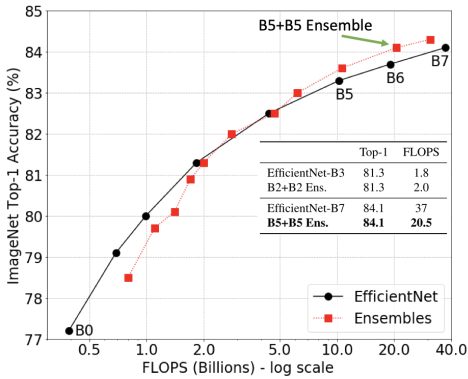
Despite the success and widespread adoption of smartphones, using them to compose longer pieces of text is still quite cumbersome. As one writes, grammatical errors can often creep into the text (especially undesirable in formal situations), and correcting these errors can be time consuming on a small display with limited controls.

To address some of these challenges, we are launching a grammar correction feature that is directly built into Gboard on Pixel 6 that works entirely on-device to preserve privacy, detecting and suggesting corrections for grammatical errors while the user is typing. Building such functionality required addressing a few key obstacles: memory size limitations, latency requirements, and handling partial sentences. Currently, the feature is capable of correcting English sentences (we plan to expand to more languages in the near future) and available on almost any app with Gboard¹.

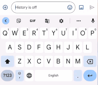Gboard suggests how to correct an ungrammatical sentence as the user types.

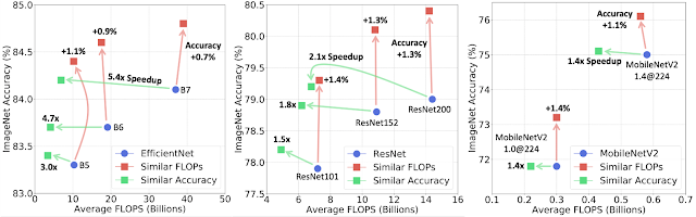
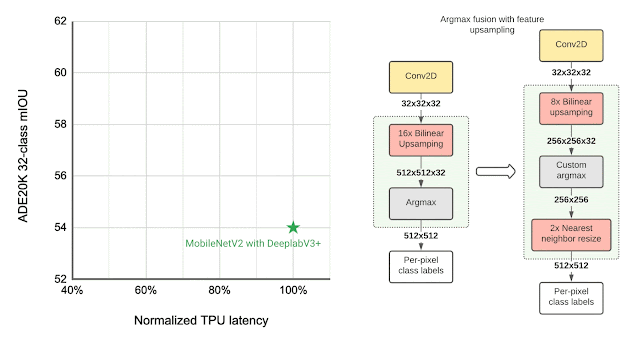
Model Architecture
We trained a sequence-to-sequence neural network to take an input sentence (or a sentence prefix) and output the grammatically correct version — if the original text is already grammatically correct, the output of the model is identical to its input, indicating that no corrections are needed. The model uses a hybrid architecture that combines a Transformer encoder with an LSTM decoder, a combination that provides a good balance of quality and latency.

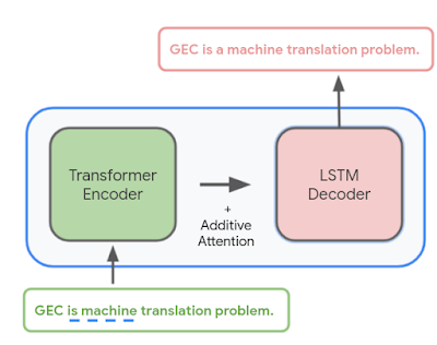Overview of the grammatical error correction (GEC) model architecture.

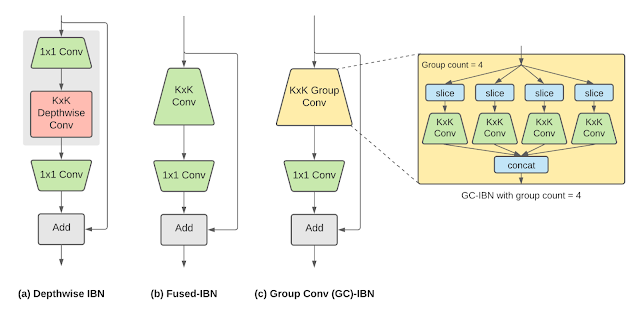
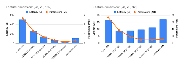
Mobile devices are constrained by limited memory and computational power, which make it more difficult to build a high quality grammar checking system. There are a few techniques we use to build a small, efficient, and capable model.

• Shared embedding: Because the input and output of the model are structurally similar (e.g., both are text in the same language), we share some of the model weights between the Transformer encoder and the LSTM decoder, which reduces the model file size considerably without unduly affecting accuracy.
• Factorized embedding: The model splits a sentence into a sequence of predefined tokens. To achieve good quality, we find that it is important to use a large vocabulary of predefined tokens, however, this substantially increases the model size. A factorized embedding separates the size of the hidden layers from the size of the vocabulary embedding. This enables us to have a model with a large vocabulary without significantly increasing the number of total weights.
• Quantization: To reduce the model size further, we perform post-training quantization, which allows us to store each 32-bit floating point weight using only 8-bits. While this means that each weight is stored with lower fidelity, nevertheless, we find that the quality of the model is not materially affected.

By employing these techniques, the resulting model takes up only 20MB of storage and performs inference on 60 input characters under 22ms on the Google Pixel 6 CPU.

Training the Model
In order to train the model, we needed training data in the form of <original, corrected> text pairs.

One possible approach to generating a small on-device model would be to use the same training data as a large cloud-based grammar model. While this data produces a reasonably high quality on-device model, we found that using a technique called hard distillation to generate training data that is better-matched to the on-device domain yields even better quality results.

Hard distillation works as follows: We first collected hundreds of millions of English sentences from across the public web. We then used the large cloud-based grammar model to generate grammar corrections for those sentences. This training dataset of <original, corrected> sentence pairs is then used to train a smaller on-device model that can correct full sentences. We found that the on-device model built from this training dataset produces significantly higher quality suggestions than a similar-sized on-device model built on the original data used to train the cloud-based model.

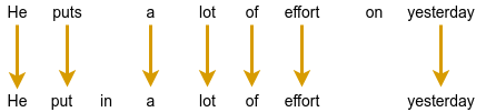
Before training the model from this data, however, there is another issue to address. To enable the model to correct grammar as the user types (an important capability of mobile devices) it needs to be able to handle sentence prefixes. While this enables grammar correction when the user has only typed part of a sentence, this capability is particularly useful in messaging apps, where the user often omits the final period in a sentence and presses the send button as soon as they finish typing. If grammar correction is only triggered on complete sentences, it might miss many errors.

This raises the question of how to decide whether a given sentence prefix is grammatically correct. We used a heuristic to solve this — if a given sentence prefix can be completed to form a grammatically correct sentence, we then consider it grammatically correct. If not, it is assumed to be incorrect.

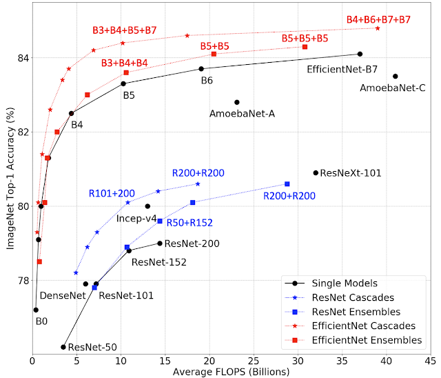
What the user has typed so far		Suggested grammar correction
She puts a lot
She puts a lot of
She puts a lot of effort
She puts a lot of effort yesterday		Replace “puts” with “put in”.

GEC on incomplete sentences. There is no correction for valid sentence prefixes.

We created a second dataset suitable for training a large cloud-based model, but this time focusing on sentence prefixes. We generated the data using the aforementioned heuristic by taking the <original, corrected> sentence pairs from the cloud-based model’s training dataset and randomly sampling aligned prefixes from them.

For example, given the <original, corrected> sentence pair:

Original sentence: She puts a lot of effort yesterday afternoon.
Corrected sentence: She put in a lot of effort yesterday afternoon.

We might sample the following prefix pairs:

Original prefix: She puts
Corrected prefix: She put in

Original prefix: She puts a lot of effort yesterday
Corrected prefix: She put in a lot of effort yesterday

We then autocompleted each original prefix to a full sentence using a neural language model (similar in spirit to that used by SmartCompose). If a full-sentence grammar model finds no errors in the full sentence, then that means there is at least one possible way to complete this original prefix without making any grammatical errors, so we consider the original prefix to be correct and output <original prefix, original prefix> as a training example. Otherwise, we output <original prefix, corrected prefix>. We used this training data to train a large cloud-based model that can correct sentence prefixes, then used that model for hard distillation, generating new <original, corrected> sentence prefix pairs that are better-matched to the on-device domain.

Finally, we constructed the final training data for the on-device model by combining these new sentence prefix pairs with the full sentence pairs. The on-device model trained on this combined data is then capable of correcting both full sentences as well as sentence prefixes.

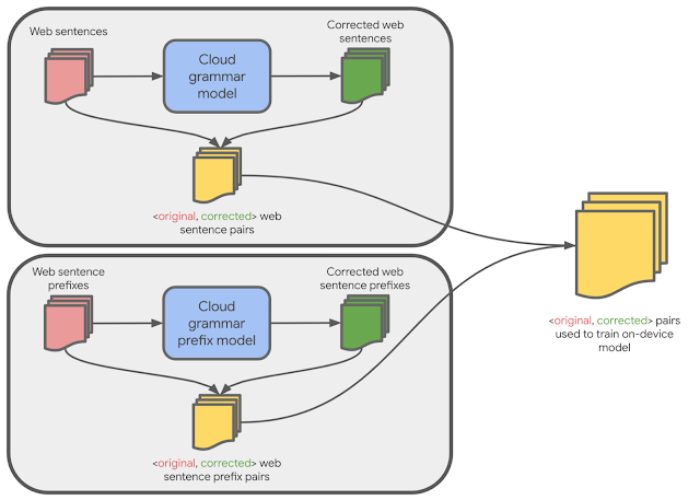Training data for the on-device model is generated from cloud-based models.

Grammar Correction On-Device
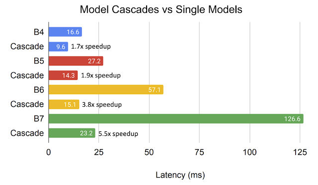
Gboard sends a request to the on-device grammar model whenever the user has typed more than three words, whether the sentence is completed or not. To provide a quality user experience, we underline the grammar mistakes and provide replacement suggestions when the user interacts with them. However, the model outputs only corrected sentences, so those need to be transformed into replacement suggestions. To do this, we align the original sentence and the corrected sentence by minimizing the Levenshtein distance (i.e., the number of edits that are needed to transform the original sentence to the corrected sentence).

Extracting edits by aligning the corrected sentence to the original sentence.

Finally, we transform the insertion edits and deletion edits to be replacement edits. In the above example, we transform the suggested insertion of “in” to be an edit that suggests replacing “puts” with “put in”. And we similarly suggest replacing “effort on” with “effort”.

Conclusion
We have built a small high-quality grammar correction model by designing a compact model architecture and leveraging a cloud-based grammar system during training via hard distillation. This compact model enables users to correct their text entirely on their own device without ever needing to send their keystrokes to a remote server.

Acknowledgements
We gratefully acknowledge the key contributions of the other team members, including Abhanshu Sharma, Akshay Kannan, Bharath Mankalale, Chenxi Ni, Felix Stahlberg, Florian Hartmann, Jacek Jurewicz, Jayakumar Hoskere, Jenny Chin, Kohsuke Yatoh, Lukas Zilka, Martin Sundermeyer, Matt Sharifi, Max Gubin, Nick Pezzotti, Nithi Gupta, Olivia Graham, Qi Wang, Sam Jaffee, Sebastian Millius, Shankar Kumar, Sina Hassani, Vishal Kumawat, and Yuanbo Zhang, Yunpeng Li, Yuxin Dai. We would also like to thank Xu Liu and David Petrou for their support.

---

¹The feature will eventually be available in all apps with Gboard, but is currently unavailable for those in WebView. ^↩

Posted by Xiaofang Wang, Intern and Yair Alon (prev. Movshovitz-Attias), Software Engineer, Google Research

When building a deep model for a new machine learning application, researchers often begin with existing network architectures, such as ResNets or EfficientNets. If the initial model’s accuracy isn’t high enough, a larger model may be a tempting alternative, but may not actually be the best solution for the task at hand. Instead, better performance potentially could be achieved by designing a new model that is optimized for the task. However, such efforts can be challenging and usually require considerable resources.

In “Wisdom of Committees: An Overlooked Approach to Faster and More Accurate Models”, we discuss model ensembles and a subset called model cascades, both of which are simple approaches that construct new models by collecting existing models and combining their outputs. We demonstrate that ensembles of even a small number of models that are easily constructed can match or exceed the accuracy of state-of-the-art models while being considerably more efficient.

What Are Model Ensembles and Cascades?
Ensembles and cascades are related approaches that leverage the advantages of multiple models to achieve a better solution. Ensembles execute multiple models in parallel and then combine their outputs to make the final prediction. Cascades are a subset of ensembles, but execute the collected models sequentially, and merge the solutions once the prediction has a high enough confidence. For simple inputs, cascades use less computation, but for more complex inputs, may end up calling on a greater number of models, resulting in higher computation costs.

Overview of ensembles and cascades. While this example shows 2-model combinations for both ensembles and cascades, any number of models can potentially be used.

Compared to a single model, ensembles can provide improved accuracy if there is variety in the collected models’ predictions. For example, the majority of images in ImageNet are easy for contemporary image recognition models to classify, but there are many images for which predictions vary between models and that will benefit most from an ensemble.

While ensembles are well-known, they are often not considered a core building block of deep model architectures and are rarely explored when researchers are developing more efficient models (with a few notable exceptions [1, 2, 3]). Therefore, we conduct a comprehensive analysis of ensemble efficiency and show that a simple ensemble or cascade of off-the-shelf pre-trained models can enhance both the efficiency and accuracy of state-of-the-art models.

To encourage the adoption of model ensembles, we demonstrate the following beneficial properties:

1. Simple to build: Ensembles do not require complicated techniques (e.g., early exit policy learning).
2. Easy to maintain: Ensembles are trained independently, making them easy to maintain and deploy.
3. Affordable to train: The total training cost of models in an ensemble is often lower than a similarly accurate single model.
4. On-device speedup: The reduction in computation cost (FLOPS) successfully translates to a speedup on real hardware.

Efficiency and Training Speed
It’s not surprising that ensembles can increase accuracy, but using multiple models in an ensemble may introduce extra computational cost at runtime. So, we investigate whether an ensemble can be more accurate than a single model that has the same computational cost. We analyze a series of models, EfficientNet-B0 to EfficientNet-B7, that have different levels of accuracy and FLOPS when applied to ImageNet inputs. The ensemble predictions are computed by averaging the predictions of each individual model.

We find that ensembles are significantly more cost-effective in the large computation regime (>5B FLOPS). For example, an ensemble of two EfficientNet-B5 models matches the accuracy of a single EfficientNet-B7 model, but does so using ~50% fewer FLOPS. This demonstrates that instead of using a large model, in this situation, one should use an ensemble of multiple considerably smaller models, which will reduce computation requirements while maintaining accuracy. Moreover, we find that the training cost of an ensemble can be much lower (e.g., two B5 models: 96 TPU days total; one B7 model: 160 TPU days). In practice, model ensemble training can be parallelized using multiple accelerators leading to further reductions. This pattern holds for the ResNet and MobileNet families as well.

Ensembles outperform single models in the large computation regime (>5B FLOPS).

Power and Simplicity of Cascades
While we have demonstrated the utility of model ensembles, applying an ensemble is often wasteful for easy inputs where a subset of the ensemble will give the correct answer. In these situations, cascades save computation by allowing for an early exit, potentially stopping and outputting an answer before all models are used. The challenge is to determine when to exit from the cascade.

To highlight the practical benefit of cascades, we intentionally choose a simple heuristic to measure the confidence of the prediction — we take the confidence of the model to be the maximum of the probabilities assigned to each class. For example, if the predicted probabilities for an image being either a cat, dog, or horse were 20%, 80% and 20%, respectively, then the confidence of the model’s prediction (dog) would be 0.8. We use a threshold on the confidence score to determine when to exit from the cascade.

To test this approach, we build model cascades for the EfficientNet, ResNet, and MobileNetV2 families to match either computation costs or accuracy (limiting the cascade to a maximum of four models). By design in cascades, some inputs incur more FLOPS than others, because more challenging inputs go through more models in the cascade than easier inputs. So we report the average FLOPS computed over all test images. We show that cascades outperform single models in all computation regimes (when FLOPS range from 0.15B to 37B) and can enhance accuracy or reduce the FLOPS (sometimes both) for all models tested.

Cascades of EfficientNet (left), ResNet (middle) and MobileNetV2 (right) models on ImageNet. When using similar FLOPS, cascades obtain a higher accuracy than single models (shown by the red arrows pointing up). Cascades can also match the accuracy of single models with significantly fewer FLOPS e.g., 5.4x for B7 (green arrows pointing left).

Summary of accuracy vs. FLOPS for ensembles and cascades. Squares and stars represent ensembles and cascades, respectively,, and the “+” notation indicates the models that comprise the ensemble or cascade. For example, ”B3+B4+B5+B7” at a star refers to a cascade of EfficientNet-B3, B4, B5 and B7 models.

In some cases it is not the average computation cost but the worst-case cost that is the limiting factor. By adding a simple constraint to the cascade building procedure, one can guarantee an upper bound to the computation cost of the cascade. See the paper for more details.

Other than convolutional neural networks, we also consider a Transformer-based architecture, ViT. We build a cascade of ViT-Base and ViT-Large models to match the average computation or accuracy of a single state-of-the-art ViT-Large model, and show that the benefit of cascades also generalizes to Transformer-based architectures.

	Single Models		Cascades – Similar Throughput			Cascades – Similar Accuracy
	Top-1 (%)	Throughput	Top-1 (%)	Throughput	△Top-1	Top-1 (%)	Throughput	SpeedUp
ViT-L-224	82.0	192	83.1	221	1.1	82.3	409	2.1x
ViT-L-384	85.0	54	86.0	69	1.0	85.2	125	2.3x

Cascades of ViT models on ImageNet. “224” and “384” indicate the image resolution on which the model is trained. Throughput is measured as the number of images processed per second. Our cascades can achieve a 1.0% higher accuracy than ViT-L-384 with a similar throughput or achieve a 2.3x speedup over that model while matching its accuracy.

Earlier works on cascades have also shown efficiency improvements for state-of-the-art models, but here we demonstrate that a simple approach with a handful of models is sufficient.

Inference Latency
In the above analysis, we average FLOPS to measure the computational cost. It is also important to verify that the FLOPS reduction obtained by cascades actually translates into speedup on hardware. We examine this by comparing on-device latency and speed-up for similarly performing single models versus cascades. We find a reduction in the average online latency on TPUv3 of up to 5.5x for cascades of models from the EfficientNet family compared to single models with comparable accuracy. As models become larger the more speed-up we find with comparable cascades.

Average latency of cascades on TPUv3 for online processing. Each pair of same colored bars has comparable accuracy. Notice that cascades provide drastic latency reduction.

Building Cascades from Large Pools of Models
Above, we limit the model types and only consider ensembles/cascades of at most four models. While this highlights the simplicity of using ensembles, it also allows us to check all combinations of models in very little time so we can find optimal model collections with only a few CPU hours on a held out set of predictions.

When a large pool of models exists, we would expect cascades to be even more efficient and accurate, but brute force search is not feasible. However, efficient cascade search methods have been proposed. For example, the algorithm of Streeter (2018), when applied to a large pool of models, produced cascades that matched the accuracy of state-of-the-art neural architecture search–based ImageNet models with significantly fewer FLOPS, for a range of model sizes.

Conclusion
As we have seen, ensemble/cascade-based models obtain superior efficiency and accuracy over state-of-the-art models from several standard architecture families. In our paper we show more results for other models and tasks. For practitioners, this outlines a simple procedure to boost accuracy while retaining efficiency using off-the-shelf models. We encourage you to try it out!

Acknowledgement
This blog presents research done by Xiaofang Wang (while interning at Google Research), Dan Kondratyuk, Eric Christiansen, Kris M. Kitani, Yair Alon (prev. Movshovitz-Attias), and Elad Eban. We thank Sergey Ioffe, Shankar Krishnan, Max Moroz, Josh Dillon, Alex Alemi, Jascha Sohl-Dickstein‎, Rif A Saurous, and Andrew Helton for their valuable help and feedback.

Posted by Michael Dixon, Software Engineer and Reena Singhal Lee, Product Manager, Google Health

Earlier this year, we launched Contactless Sleep Sensing in Nest Hub, an opt-in feature that can help users better understand their sleep patterns and nighttime wellness. While some of the most critical sleep insights can be derived from a person’s overall schedule and duration of sleep, that alone does not tell the complete story. The human brain has special neurocircuitry to coordinate sleep cycles — transitions between deep, light, and rapid eye movement (REM) stages of sleep — vital not only for physical and emotional wellbeing, but also for optimal physical and cognitive performance. Combining such sleep staging information with disturbance events can help you better understand what’s happening while you’re sleeping.

Today we announced enhancements to Sleep Sensing that provide deeper sleep insights. While not intended for medical purposes¹, these enhancements allow better understanding of sleep through sleep stages and the separation of the user’s coughs and snores from other sounds in the room. Here we describe how we developed these novel technologies, through transfer learning techniques to estimate sleep stages and sensor fusion of radar and microphone signals to disambiguate the source of sleep disturbances.

To help people understand their sleep patterns, Nest Hub displays a hypnogram, plotting the user’s sleep stages over the course of a sleep session. Potential sound disturbances during sleep will now include “Other sounds” in the timeline to separate the user’s coughs and snores from other sound disturbances detected from sources in the room outside of the calibrated sleeping area.

Training and Evaluating the Sleep Staging Classification Model
Most people cycle through sleep stages 4-6 times a night, about every 80-120 minutes, sometimes with a brief awakening between cycles. Recognizing the value for users to understand their sleep stages, we have extended Nest Hub’s sleep-wake algorithms using Soli to distinguish between light, deep, and REM sleep. We employed a design that is generally similar to Nest Hub’s original sleep detection algorithm: sliding windows of raw radar samples are processed to produce spectrogram features, and these are continuously fed into a Tensorflow Lite model. The key difference is that this new model was trained to predict sleep stages rather than simple sleep-wake status, and thus required new data and a more sophisticated training process.

In order to assemble a rich and diverse dataset suitable for training high-performing ML models, we leveraged existing non-radar datasets and applied transfer learning techniques to train the model. The gold standard for identifying sleep stages is polysomnography (PSG), which employs an array of wearable sensors to monitor a number of body functions during sleep, such as brain activity, heartbeat, respiration, eye movement, and motion. These signals can then be interpreted by trained sleep technologists to determine sleep stages.

To develop our model, we used publicly available data from the Sleep Heart Health Study (SHHS) and Multi-ethnic Study of Atherosclerosis (MESA) studies with over 10,000 sessions of raw PSG sensor data with corresponding sleep staging ground-truth labels, from the National Sleep Research Resource. The thoracic respiratory inductance plethysmography (RIP) sensor data within these PSG datasets is collected through a strap worn around the patient’s chest to measure motion due to breathing. While this is a very different sensing modality from radar, both RIP and radar provide signals that can be used to characterize a participant’s breathing and movement. This similarity between the two domains makes it possible to leverage a plethysmography-based model and adapt it to work with radar.

To do so, we first computed spectrograms from the RIP time series signals and used these as features to train a convolutional neural network (CNN) to predict the groundtruth sleep stages. This model successfully learned to identify breathing and motion patterns in the RIP signal that could be used to distinguish between different sleep stages. This indicated to us that the same should also be possible when using radar-based signals.

To test the generality of this model, we substituted similar spectrogram features computed from Nest Hub’s Soli sensor and evaluated how well the model was able to generalize to a different sensing modality. As expected, the model trained to predict sleep stages from a plethysmograph sensor was much less accurate when given radar sensor data instead. However, the model still performed much better than chance, which demonstrated that it had learned features that were relevant across both domains.

To improve on this, we collected a smaller secondary dataset of radar sensor data with corresponding PSG-based groundtruth labels, and then used a portion of this dataset to fine-tune the weights of the initial model. This smaller amount of additional training data allowed the model to adapt the original features it had learned from plethysmography-based sleep staging and successfully generalize them to our domain. When evaluated on an unseen test set of new radar data, we found the fine-tuned model produced sleep staging results comparable to that of other consumer sleep trackers.

The custom ML model efficiently processes a continuous stream of 3D radar tensors (as shown in the spectrogram at the top of the figure) to automatically compute probabilities of each sleep stage — REM, light, and deep — or detect if the user is awake or restless.

More Intelligent Audio Sensing Through Audio Source Separation
Soli-based sleep tracking gives users a convenient and reliable way to see how much sleep they are getting and when sleep disruptions occur. However, to understand and improve their sleep, users also need to understand why their sleep may be disrupted. We’ve previously discussed how Nest Hub can help monitor coughing and snoring, frequent sources of sleep disturbances of which people are often unaware. To provide deeper insight into these disturbances, it is important to understand if the snores and coughs detected are your own.

The original algorithms on Nest Hub used an on-device, CNN-based detector to process Nest Hub’s microphone signal and detect coughing or snoring events, but this audio-only approach did not attempt to distinguish from where a sound originated. Combining audio sensing with Soli-based motion and breathing cues, we updated our algorithms to separate sleep disturbances from the user-specified sleeping area versus other sources in the room. For example, when the primary user is snoring, the snoring in the audio signal will correspond closely with the inhalations and exhalations detected by Nest Hub’s radar sensor. Conversely, when snoring is detected outside the calibrated sleeping area, the two signals will vary independently. When Nest Hub detects coughing or snoring but determines that there is insufficient correlation between the audio and motion features, it will exclude these events from the user’s coughing or snoring timeline and instead note them as “Other sounds” on Nest Hub’s display. The updated model continues to use entirely on-device audio processing with privacy-preserving analysis, with no raw audio data sent to Google’s servers. A user can then opt to save the outputs of the processing (sound occurrences, such as the number of coughs and snore minutes) in Google Fit, in order to view their night time wellness over time.

Snoring sounds that are synchronized with the user’s breathing pattern (left) will be displayed in the user’s Nest Hub’s Snoring timeline. Snoring sounds that do not align with the user’s breathing pattern (right) will be displayed in Nest Hub’s “Other sounds” timeline.

Since Nest Hub with Sleep Sensing launched, researchers have expressed interest in investigational studies using Nest Hub’s digital quantification of nighttime cough. For example, a small feasibility study supported by the Cystic Fibrosis Foundation² is currently underway to evaluate the feasibility of measuring night time cough using Nest Hub in families of children with cystic fibrosis (CF), a rare inherited disease, which can result in a chronic cough due to mucus in the lungs. Researchers are exploring if quantifying cough at night could be a proxy for monitoring response to treatment.

Conclusion
Based on privacy-preserving radar and audio signals, these improved sleep staging and audio sensing features on Nest Hub provide deeper insights that we hope will help users translate their night time wellness into actionable improvements for their overall wellbeing.

Acknowledgements
This work involved collaborative efforts from a multidisciplinary team of software engineers, researchers, clinicians, and cross-functional contributors. Special thanks to Dr. Logan Schneider, a sleep neurologist whose clinical expertise and contributions were invaluable to continuously guide this research. In addition to the authors, key contributors to this research include Anupam Pathak, Jeffrey Yu, Arno Charton, Jian Cui, Sinan Hersek, Jonathan Hsu, Andi Janti, Linda Lei, Shao-Po Ma, ‎Jo Schaeffer, Neil Smith, Siddhant Swaroop, Bhavana Koka, Dr. Jim Taylor, and the extended team. Thanks to Mark Malhotra and Shwetak Patel for their ongoing leadership, as well as the Nest, Fit, and Assistant teams we collaborated with to build and validate these enhancements to Sleep Sensing on Nest Hub.

---

¹Not intended to diagnose, cure, mitigate, prevent or treat any disease or condition. ^↩
2Google did not have any role in study design, execution, or funding. ^↩