Hello, so I am currently trying to learn TensorFlow and deep learning this month since we have an upcoming thesis proposal next semester and I am somewhat interested in proposing a thesis that will implement machine learning in it. To be specific, my envisioned thesis proposal will be about the early detection of pests in plants so that there will be a way for farmers to somewhat predict the conditions of their crops. I think that image recognition using machine learning can help me with this since I have read that there are a lot of things image recognition can do. Although my knowledge about machine learning and AI is very futile, especially the details in it like the Math involved and creating my own model from scratch for implementation of my envisioned topic. Tho I have heard from my colleagues, which were like me that has a proposal that involves machine learning and started doing their thesis with zero knowledge about it, that there are lots of open-source models available on the internet which can help me implement my proposal. Actually, they themselves used open-source models (which implement R-CNN and YOLO algorithms) in implementing their proposal, which I think is about microplastic detection in bodies of water using image recognition. What they’ve done is they formulated and populated their own datasets about it, the gathered dataset was used to train the model they got from the internet, tho they made some tweaking.
So my concern here is that, given my prospective proposal, should I in-depth learn about TensorFlow and create a model from scratch (which actually is good since I will learn the fundamentals about ML but it will require me a lot of effort) or just try to learn open-source models available on the internet then try to tweak something in it to best fit my intended function. I am currently taking a course in Udacity which is an Intro to Tensorflow for Deep Learning, this was the prescribed overview course of the tensorflow website, and I am somewhat unsatisfied by how things worked on that course since the course somewhat bombards me of all the codes and stuff which I really don’t know since I am new to TensorFlow (tho I know things in python). They did not give such an in-depth explanation of the codes although they give somewhat a crash course on different Deep Learning concepts such as CNNs. I am overwhelmed by that course since what I just did is to follow the tutorial, actually, I just push the play button in the google colab and wait for it to run and see if its working as intended just like what’s shown in the video tutorial. I know I am expecting a lot from that course knowing that it is an overview of the ML and TF, but I am really not satisfied with what I am getting. I want to know more about Tensorflow, especially the library itself and the codes involved, I think learning the code itself while learning the concepts involved will help me grow in this field. So are there any recommendations on which resources should I gather and learn to satisfy my learning needs in this field? Also, what better ways (I actually love getting advice from people who are better than me in this field) to learn ML and TF. I am looking forward to having a good conversation with you guys and also learning a lot about this field.
submitted by /u/MapDiscombobulated65
[visit reddit] [comments]

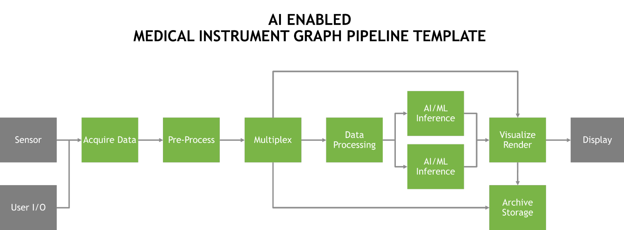
 Clara Holoscan SDK 0.2 offers real-time AI inference capabilities and fast I/O for high-performance streaming applications in medical devices.
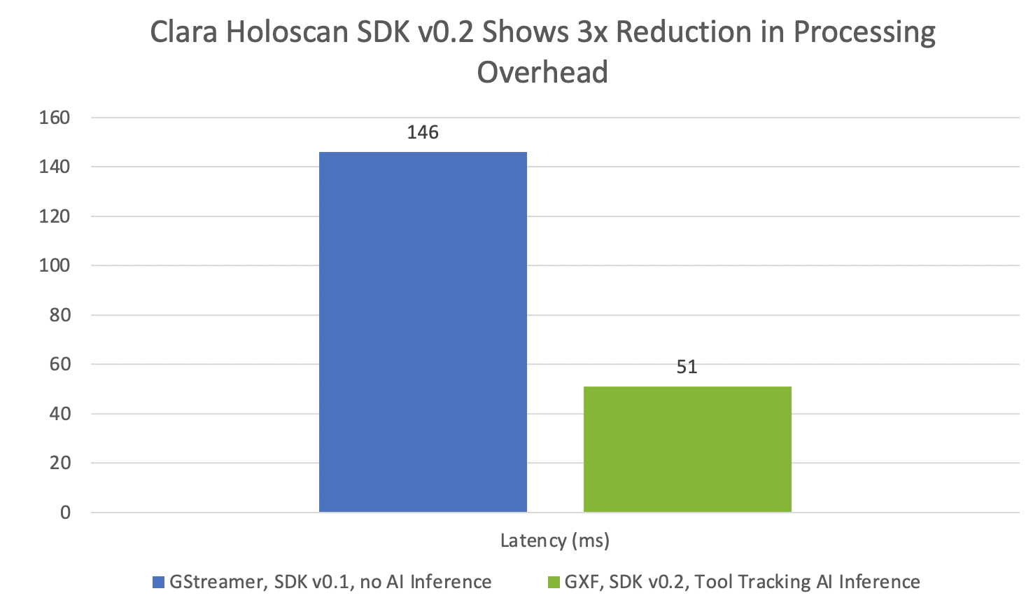
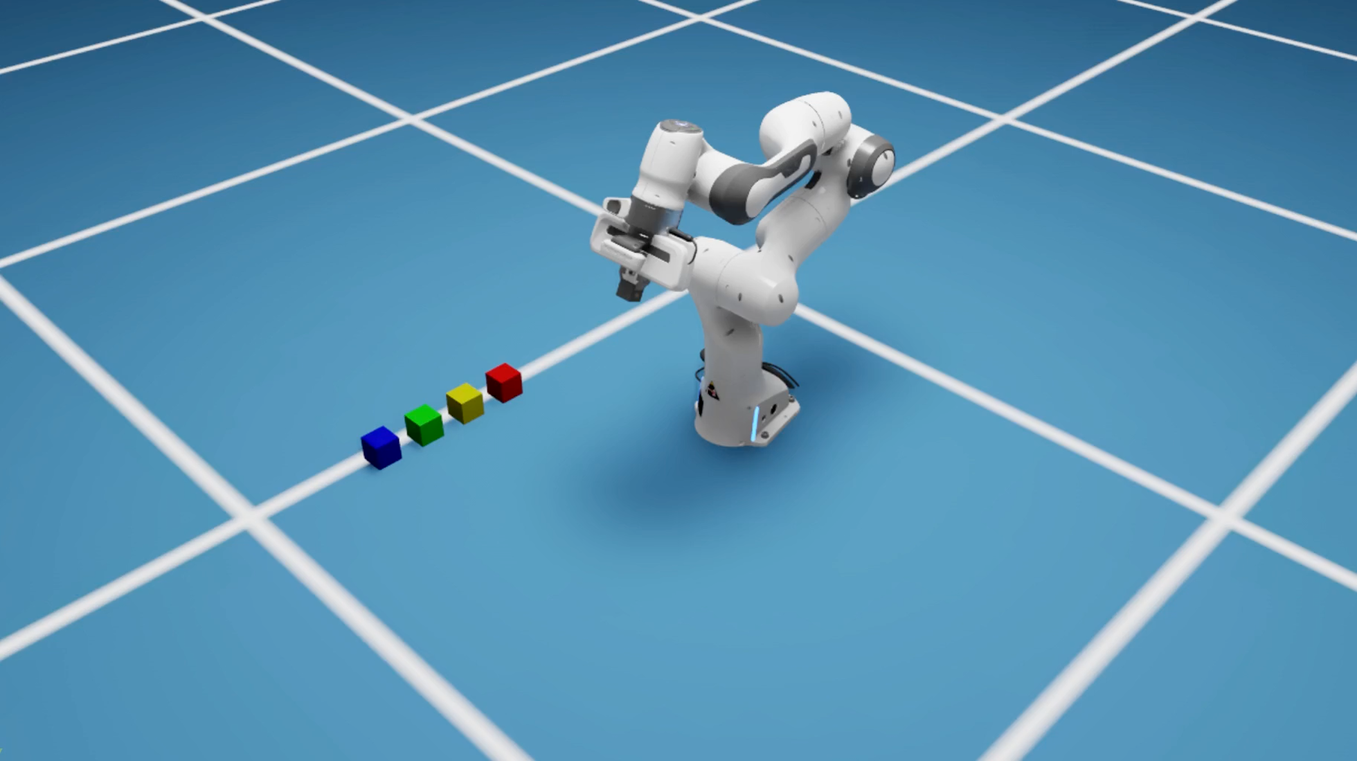
 This release of Isaac Sim adds more tools for AI-based robotics including Isaac Gym support for RL, Isaac Cortex for cobot programming, and much more.