DataBloom

Using NVIDIA TAO Toolkit and Innotescus’ data curation and analysis platform to improve a popular object detection model’s performance on the person class by over 20%.

AI applications are powered by machine learning models that are trained to predict outcomes accurately based on input data such as images, text, or audio. Training a machine learning model from scratch requires vast amounts of data and a considerable amount of human expertise, often making the process too expensive and time-consuming for most organizations.

Transfer learning is the happy medium between building a custom model from scratch and choosing an off-the-shelf commercial model to integrate into an ML application. With transfer learning, you can select a pretrained model that’s related to your solution and retrain it on data reflecting your specific use case. Transfer learning strikes the right balance between the custom-everything approach (often too expensive)  and an off-the-shelf approach (often too rigid) and enables you to build tailored solutions with fewer resources.

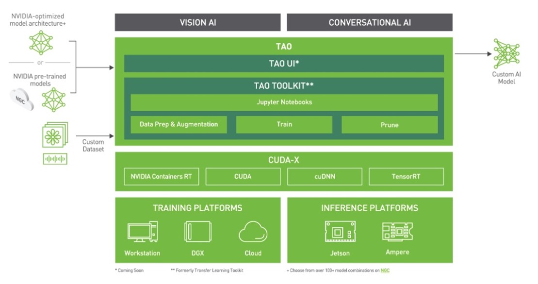
The NVIDIA TAO Toolkit enables you to apply transfer learning to pretrained models and create custom, production-ready models without the complexity of AI frameworks. To train these models, high-quality data is a must. While TAO focuses on the model-centric steps of the development process, Innotescus focuses on the data-centric steps. 

Innotescus is a web-based platform for annotating, analyzing, and curating robust, unbiased datasets for computer vision–based machine learning. Innotescus helps teams scale operations without sacrificing quality. The platform includes automated and assisted annotation for both images and videos, consensus and review features for QA processes, and interactive analytics for proactive dataset analysis and balancing. Together, Innotescus and the TAO toolkit make it cost effective for organizations to apply transfer learning successfully in custom applications, arriving at high performing solutions in little time.

In this post, we address the challenges of building a robust object detection model by integrating the NVIDIA TAO Toolkit with Innotescus. This solution alleviates several common pain points that businesses encounter when building and deploying commercial solutions.

YOLO object detection model

Your goal in this project is to apply transfer learning to the YOLO object detection model in the TAO toolkit using data curated on Innotescus.

Object detection is the ability to localize and classify objects with a bounding box in an image or video. It is the most widely used application of computer vision technology. Object detection solves many complex, real-world challenges, such as the following:

• Context and scene understanding
• Automating solutions for smart retail
• Autonomous driving
• Precision agriculture

Why should you use YOLO for this model? Traditionally, deep learning–based object detectors operate through a two-stage process. In the first stage, the model identifies regions of interest in an image. In the second stage, each of these regions are classified.

Typically, many regions are sent to the classification stage, and because classification is an expensive operation, two-stage object detectors are extremely slow. YOLO stands for “You only look once.” As the name suggests, YOLO can localize and classify simultaneously, leading to highly accurate real-time performance, which is essential for most deployable solutions. In April 2020, the fourth iteration of YOLO was published. It has been tested on a multitude of applications and industries and has proven to be robust. 

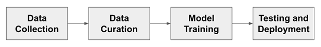
Figure 1 shows the general pipeline for training object detection models. For each step of this more traditional development pipeline, we discuss the typical challenges that people encounter and how the combination of TAO and Innotescus solves these problems.

Before you begin, install the TAO toolkit and authenticate your instance of the Innotescus API.

Installing TAO Toolkit

The TAO toolkit can be run as a CLI or in a Jupyter notebook. It’s only compatible with Python3 (3.6.9 and 3.7), so first install the prerequisites.

Install docker-ce.

• On Linux, check the post-installation steps to ensure that Docker can be run without sudo.
• Install nvidia-container-toolkit.
• Create an NGC account and generate an API key for authentication.
• Log in to the NGC Docker registry by running the command docker login nvcr.io and enter your credentials for authentication.

After the prerequisites are installed, install the TAO toolkit. NVIDIA recommends installing the package in a virtual environment using virtualenvwrapper. To install the TAO launcher Python package, run the following commands:

pip3 install nvidia-pyindex
pip3 install nvidia-tao

Check whether you’ve gone through the installation correctly by running tao --help.

Accessing the Innotescus API

Innotescus is accessible as a web-based application, but you’ll also use its API to demonstrate how to accomplish the same tasks programmatically. To begin, install the Innotescus library.

pip install innotescus

Next, authenticate the API instance using the client_id and client_secret values retrieved from the platform.

from innotescus import client_factory
client = client_factory(client_id=’client_id’, client_secret=’client_secret’)

Now you’re ready to interact with the platform through the API, which you’ll do as you walk through each step of the pipeline that follows.

Data collection

You need data to train the model. Though it’s often overlooked, data collection is arguably the most important step in the development process. While collecting data, you should ask yourself a few questions:

• Is the training data adequately representative of each object of interest?
• Are you accounting for all the scenarios in which you expect the model to be deployed?
• Do you have enough data to train the model?

You can’t always answer these questions completely but having a well-rounded game plan for data collection helps you avoid issues during subsequent steps in the development process. Data collection is a time-consuming and expensive process. Because the models provided by TAO are pretrained, the data requirements for retraining are much smaller, saving organizations significant resources in this phase.

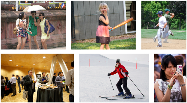
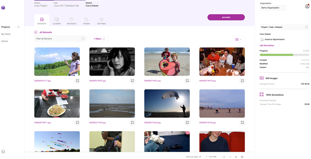
For this experiment, you use images and annotations from the MS COCO Validation 2017 dataset. This dataset has 5,000 images with 80 different classes, but you only use the 2,685 images containing at least one person.

%matplotlib inline
from pycocotools.coco import COCO
import matplotlib.pyplot as plt

dataDir=’Your Data Directory’
dataType=’val2017’
annFile=’{}/annotations/instances_{}.json’.format(dataDir,dataType)

coco=COCO(annFile)

catIds = coco.getCatIds(catNms=[‘person’]) # only using ‘person’ category
imgIds = coco.getImgIds(catIds=catIds)

for num_imgs in len(imgIds): 
	img = coco.loadImgs(imgIds[num_imgs])[0]
	I = io.imread(img[‘coco_url’])

With the authenticated instance of the Innotescus client, begin setting up a project and uploading the human-focused dataset.

#create a new project
client.create_project(project_name)
#upload data to the new project
client.upload_data(project_name, dataset_name, file_paths, data_type, storage_type)

• data_type: The type of data this dataset holds. Accepted values:
  • DataType.IMAGE
  • DataType.VIDEO
• storage_type: The source of the data. Accepted values:
  • StorageType.FILE_SYSTEM
  • StorageType.URL

This dataset is now accessible through the Innotescus user interface.

Data curation

Now that you have your initial dataset, begin curating it to ensure a well-balanced dataset. Studies have repeatedly shown that this phase of the process takes around 80% of the time spent on a machine learning project.

Using TAO and Innotescus, we highlight techniques like pre-annotation and review that save time during this step without sacrificing dataset size or quality.

Pre-annotation

Pre-annotation enables you to use model-generated annotations to remove a significant amount of the time and manual effort necessary to label the subset of 2,685 images accurately. You use YOLOv4—the same model that you’re retraining—to generate pre-annotations for the annotators to refine.

Because pre-annotation saves you so much time on the easier components of the annotation task, you can focus your attention on the harder examples that the model can’t yet handle.

YOLOv4 is included in the TAO toolkit and supports k-means clustering, training, evaluation, inference, pruning, and exporting. To use the model, you must first create a YOLOv4 spec file, which has the following major components:

• yolov4_config
• training_config
• eval_config
• nms_config
• augmentation_config
• dataset_config

The spec file is a protobuf text (prototxt) message, and each of its fields can be either a basic data type or a nested message.

Next, download the model with pretrained weights. The TAO Toolkit Docker container provides access to a repository of pretrained models that serve as a great starting point when training deep neural networks. Because these models are hosted on the NGC catalog, you must first download and install the NGC CLI. For more information, see the NGC documentation.

After you’ve installed the CLI, you can see the list of pretrained computer vision models on the NGC repo, and download pretrained models.

ngc registry model list nvidia/tao/pretrained_*
ngc registry model download-version /path/to/model_on_NGC_repo/ -dest /path/to/model_download_dir/

With the model downloaded and spec file updated, you can now generate pre-annotations by running the inference subtask.

tao yolo_v4 inference [-h] -i /path/to/imgFolder/ -l /path/to/annotatedOutput/ -e /path/to/specFile.txt -m /path/to/model/ -k $KEY

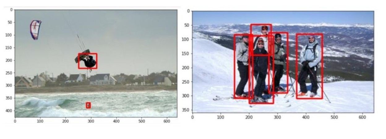
The output of the inference subtask is a series of annotations in the KITTI format, saved in the specified output directory. Figure 6 shows two examples of these annotations:

Upload the preannotations into the Innotescus platform manually through the web-based user interface or using the API. Because the KITTI format is one of the many accepted by Innotescus, no preprocessing is needed.

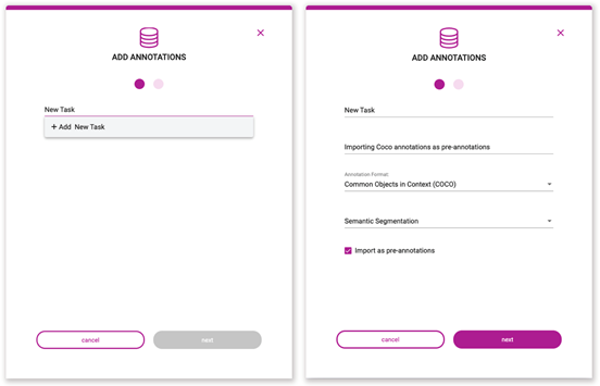
#upload pre-annotations generated by YOLOv4
Response = client.upload_annotations(project_name, dataset_name, task_type, data_type, annotation_format, file_paths, task_name, task_description, overwrite_existing_annotations, pre_annotate)

• project_name: The name of the project containing the affected dataset and task.
• dataset_name: The name of the dataset to which these annotations are to be applied.
• task_type: The type of annotation task being created with these annotations. Accepted values from the TaskType class:
  • CLASSIFICATION
  • OBJECT_DETECTION
  • SEGMENTATION
  • INSTANCE_SEGMENTATION
• data_type: The type of data to which the annotations correspond. Accepted values:
  • DataType.IMAGE
  • DataType.VIDEO
• annotation_format: The format in which these annotations are stored. Accepted values from the AnnotationFormat class:

  • COCO
  • KITTI
  • MASKS_PER_CLASS
  • PASCAL
  • CSV
  • MASKS_SEMANTIC
  • MASKS_INSTANCE
  • INNOTESCUS_JSON
  • YOLO_DARKNET
  • YOLO_KERAS
• file_paths: A list of file paths containing the annotation files to upload.
• task_name: The name of the task to which these annotations belong; if the task does not exist, it is created and populated with these annotations.
• task_description: A description of the task being created, if the task does not exist yet.
• overwrite_existing_annotations: If the task already exists, this flag allows you to overwrite existing annotations.
• pre_annotate: Allows you to import annotations as pre-annotations.

With the pre-annotations imported to the platform and a significant amount of the initial annotation work saved, move into Innotescus to further correct, refine, and analyze the data.

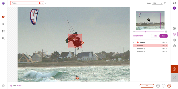
Review and correction

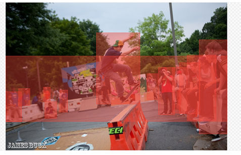
With the pre-annotations successfully imported, head over to the platform to perform review and correction of the pre-annotations. While the pretrained model saves a significant amount of annotation time, it’s still not perfect and needs a bit of human in the loop interaction to ensure high-quality training data. Figure 8 shows an example of a typical correction that you might make.

Beyond a first pass at fixing and submitting pre-annotations, Innotescus enables a more focused sampling of images and annotations for multistage review. This enables large teams to ensure high quality throughout the dataset systematically and efficiently.

Exploratory data analysis

Exploratory data analysis, or EDA, is the process of investigating and visualizing datasets from multiple statistical angles to get a holistic understanding of the underlying patterns, anomalies, and biases present in the data. It is an effective and necessary step to take before thoughtfully addressing the statistical imbalances your dataset contains.

Innotescus provides precalculated metrics for understanding class, color, spatial, and complexity distributions for both data and annotations, and enables you to add your own layer of information in image and annotation metadata to incorporate application-specific information into the analytics.

Here’s how you can use the Innotescus’s dive visualization to understand some of the patterns and biases present in the dataset. The following scatter plot shows the distribution of image entropy, which is the average information or degree of randomness in an image, within the dataset along the x-axis. You can see a clear pattern, but you can also spot anomalies like images with low entropy or information content.

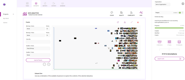
Outliers like these raise questions of how to handle anomalies within a dataset. Recognizing anomalies enables you to ask some crucial questions:

• Do you expect the model, when deployed, to encounter low-entropy input?
• If so, do you need more such examples in the training dataset?
• If not, are these examples going to be detrimental for training, and should they be removed from the training dataset?

In another example, look at each annotation’s area, relative to the image that it’s in.

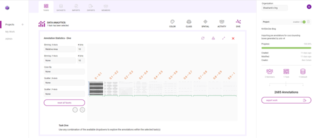
In Figure 13, the two images show the variation in annotation sizes within the dataset. While some annotations capture people that take up lots of the image, most show people far away from the camera.

Here, a large percentage of annotations are between 0 and 10% of their respective image sizes. This means that the dataset is biased towards small objects, or people that are far from the camera. Do you then need more examples in the training data that have larger annotations to represent people closer to the camera? Understanding the data distribution in this way helps you to begin thinking about the plan for data augmentation.

With Innotescus, EDA is made intuitive. It provides you with the information that you need to make powerful augmentations to your dataset and eliminate bias early in the development process.

Cluster rebalancing with dataset augmentation

The idea behind augmentation for cluster rebalancing is powerful. This technique showed a 21% boost in performance in the recent datacentric AI competition hosted by Andrew Ng and DeepLearning.AI.

You generate an N-dimensional feature vector for each data point (each bounding box annotation), and cluster all data points in higher dimensional space. When you cluster objects with similar features, you augment the dataset such that each cluster has equal representation.

We chose to use [red channel mean, green channel mean, blue channel mean, gray image std, gray image entropy, relative area] as the N-dimensional feature vector. These metrics were exported from Innotescus, which automatically calculated them. You could also use the embeddings generated by the pretrained model to populate the feature vector, which would arguably be more robust.

You use k-means clustering with k=4 as the clustering algorithm and UMAP for reducing the dimensions to two for visualization. The following code example generates the graph that shows the UMAP plot, color-coded with these four clusters.

import umap
from sklearn.decomposition import PCA
from sklearn.cluster import KMeans

# k-means on the feature vector
kmeans = KMeans(n_clusters=4, random_state=0).fit(featureVector)

# UMAP for dim reduction and visualization
fit = umap.UMAP(n_neighbors=5,
		min_dist=0.2,
		n_components=2,
		metric=’manhattan’)

u = fit.fit_transform(featureVector)

# Plot UMAP components
plt.scatter(u[:,0], u[:,1], c=(kmeans.labels_))
plt.title(‘UMAP embedding of kmeans colours’)

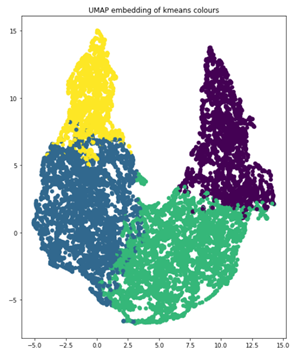
When you look at the number of objects in each cluster, you can clearly see the imbalance, which informs how you should augment the data for retraining. The four clusters represent 854, 1523, 1481 and 830 images, respectively. Where an image has objects in more than one cluster, group that image in the cluster with most of its objects for augmentation.

clusters = {}

for file, cluster in zip(filename, kmeans.labels_):
	if cluster not in clusters.keys():
		clusters[cluster] = []
		clusters[cluster].append(file)
	else:
		clusters[cluster].append(file)

for numCls in range(0, len(clusters)):
	print(‘Cluster {}: {} objects, {} images’.format(numCls+1, len(clusters[numCls]), len(list(set(clusters[numCls])))))

Output:

Cluster 1: 2234 objects, 854 images
Cluster 2: 3490 objects, 1523 images
Cluster 3: 3629 objects, 1481 images
Cluster 4: 1588 objects, 830 images

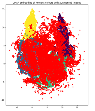
With the clusters well defined, you use the imgaug Python library to introduce augmentation techniques to enhance the training data: translation, image brightness adjustment, and scale augmentation. You augment such that each cluster contains 2,000 images for a total of 8,000. As you augment images, imgaug ensures that the annotation coordinates are altered appropriately as well.

import imgaug as ia
import imgaug.augmenters as iaa

# augment images
seq = iaa.Sequential([
	iaa.Multiply([1.1, 1.5]), # change brightness, doesn’t affect BBs
	iaa.Affine(
		translate_px={“x”:60, “y”:60},
		scale=(0.5, 0.8)
	) # translate by 60px on x/y axes & scale to 50-80%, includes BBs
])

# augment BBs and images
image_aug, bbs_aug = seq(image=I, bounding_boxes=boundingBoxes)

Using the same UMAP visualization technique, with augmented data points now in red, you see that the dataset is now much more balanced, as it more closely resembles a Gaussian distribution.

Model training

With the well-balanced, high-quality training data, the final step is to train the model.

YOLOv4 retraining on TAO Toolkit

To start retraining the model, first ensure that the spec file contains the classes of interest, as well as the correct directory paths for the pretrained model and training data. Change the training parameters in the training_config section. Reserve 30% of the augmented dataset as a test dataset to compare the performance of the pretrained model and the performance of the retrained model.

ttraining_config {
	batch_size_per_gpu: 8
	num_epochs: 80
	enable_qat: false
	checkpoint_interval: 10
	learning_rate {
		soft_start_cosine_annealing_schedule {
			min_learning_rate: 1e-7
			max_learning_rate: 1e-4
			soft_start: 0.3
		}
	}
	regularizer {
		type: L1
		weight: 3e-5
	}
	optimizer {
		adam {
			epsilon: 1e-7
			beta1: 0.9
			beta2: 0.999
			amsgrad: false
		}
	}
	pretrain_model_path: “path/to/model/model.hdf5”
}

Run the training command.

tao yolo_v4 train -e /path/to/specFile.txt -r /path/to/result -k $KEY

Results

As you can see, you achieved a 14.93% improvement in the mean average precision, a 21.37% boost from the mAP of the pretrained model:

Model	mAP50
Yolov4 pretrained model	69.86%
Yolov4 retrained model with cluster-rebalanced augmentation	84.79%

Summary

Using NVIDIA TAO Toolkit for pre-annotation and model training and Innotescus for data refinement, analysis, and curation, you improved YOLOv4’s mean average precision on the person class by a substantial amount: over 20%. Not only did you improve the performance on a selected class, you used less time and data than you would have without significant benefits of transfer learning.

Transfer learning is a great way to produce high-performing, application-specific models in settings with constrained resources. Using tools like the TAO toolkit and Innotescus makes it feasible for teams of all sizes and backgrounds.

Try it for yourself

Interested in using Innotescus to enhance and refine your own dataset? Sign up for a free trial. Get started with the TAO toolkit for your AI model training by downloading the sample resources.

Researchers combine CT imaging with deep learning to evaluate dinosaur fossils. The approach could change how paleontologists study ancient remains.

Applying new technology to studying ancient history, researchers are looking to expand their understanding of dinosaurs with a new AI algorithm. The study, published in Frontiers in Earth Science, uses high-resolution Computed Tomography (CT) imaging combined with deep learning models to scan and evaluate dinosaur fossils. The research is a step toward creating a new tool that would vastly change the way paleontologists study ancient remains. 

“Computed Tomography as well we other imaging techniques have revealed previously hidden structures in fossils, but the high-resolution images require paleontologists spending weeks to even months in post-processing, usually segmenting fossils from rock matrices. The introduction of AI can not only accelerate data processing in fossil studies, but also establish benchmarks for more objective and more reproducible studies,” said lead author Congyu Yu, a Ph.D. student at the Richard Gilder Graduate School at the American Museum of Natural History. 

For a complete picture of ancient vertebrates, paleontologists focus on internal anatomy such as cranial capacity, inner ears, or vascular spaces. To do this, researchers use a technique called thin sectioning. Removing a small piece (as thin as several micrometers) from a fossil, examining it under a microscope, and annotating the structures they find, helps them piece together the morphology of a dinosaur. However, this technique is destructive to the remains and can be extremely time consuming.

Computed tomography (CT) scans have given scientists the ability to look inside a sample while leaving the fossil unscathed. The technology essentially examines a fossil section, capturing thousands of images of it. Software then reconstructs the images and generates a three-dimensional graphic, resulting in an internal snapshot of the sample. Scientists can then examine and label identifiable morphology in the graphic to learn more about a specimen.

Imaging has given scientists a tool for revealing hidden internal structures and advancing 3D models of dinosaurs. Studies have helped researchers estimate body mass, analyze skulls, and even understand dental morphology along with tooth replacement patterns.

However, with this approach, scientists still manually choose segments, examine, and label images, which beyond being time intensive, is subjective, and can introduce errors. Plus, scans have limitations differentiating between the rock that may be coating a fossil and the bones themselves, making it difficult to determine where a rock ends and fossil begins. 

AI has proven capable of quick image segmentation in the medical world, ranging from identifying brain lesions to skin cancer. The researchers saw an opportunity to apply similar deep learning models to CT fossil images.  

They tested this new approach using deep neural networks and over 10,000 annotated CT scans of three well-preserved embryonic skulls of Protoceratop dinosaurs. Recovered in the 1990s from the Mongolian Gobi Desert, these fossils come from early horned dinosaurs and are a smaller relative of the better-known Triceratops.

The team used a classic U-net deep neural network for processing fossil segmentation, teaching the algorithm to recognize rock from the fossils. A modified DeepLab v3+ network was used for training feature identification, categorizing parts of the CT images, and 3D rendering. 

The models were trained using 7,986 manually annotated bone structure CT slices on the cuDNN-accelerated TensorFlow deep learning framework with dual NVIDIA GeForce RTX 2080 Ti GPUs.

Testing the results against a dataset of 3,329, they found that while the segmentation model reached high accuracy of around 97%, the 3D feature renderings were not as meticulous or accurate as humans. While the results showed that the features models did not perform as accurately as the scientists, the segmentation models worked smoothly and did so in record time. The models segmented each slice in seconds—manually segmenting the same piece took minutes or even hours in some cases. This could help paleontologists reduce their time spent working to differentiate fossils from rock. 

The researchers suggest that larger data sets incorporating other dinosaur species and different sediment types could help create a high-performing algorithm down the line. 

​​”We are confident that a segmentation model for fossils from the Gobi Desert is not far away, but a more generalized model needs not only more training dataset but innovations in algorithms,” Yu said in a press release. “I believe deep learning can eventually process imagery better than us, and there have already been various examples in deep learning performance exceeding humans, including Go playing and protein 3D-structure prediction.”

The dataset used in the study, CT Segmentation of Dinosaur Fossils by Deep Learning, is available for download.

Read more. >
Read the study in Frontiers in Earth Science. >>

submitted by /u/baudie
[visit reddit] [comments]

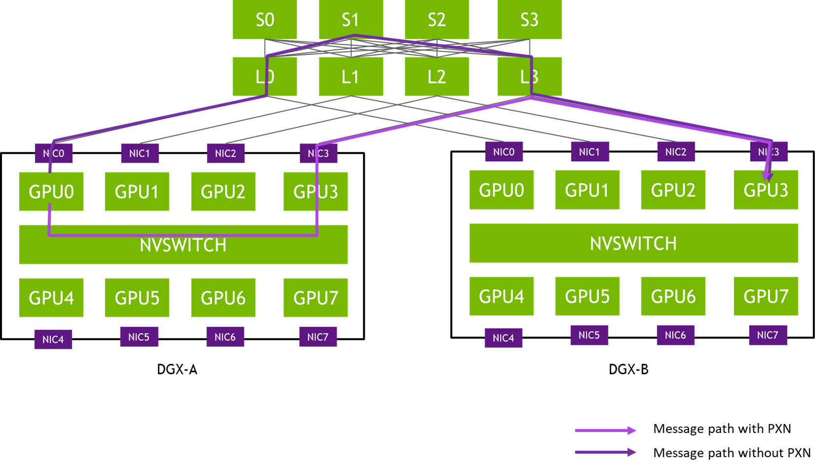
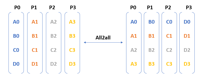
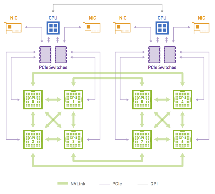
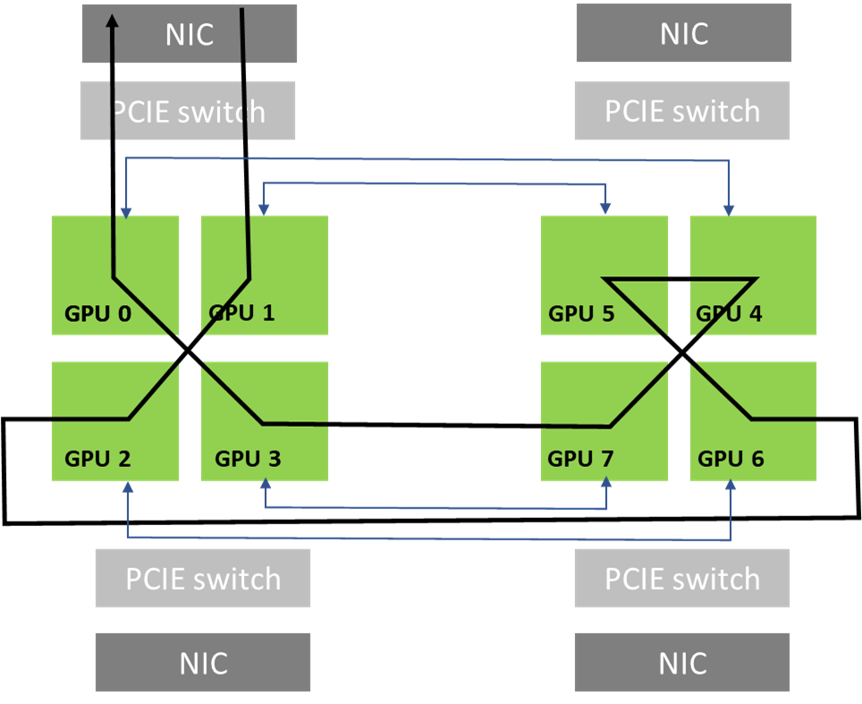
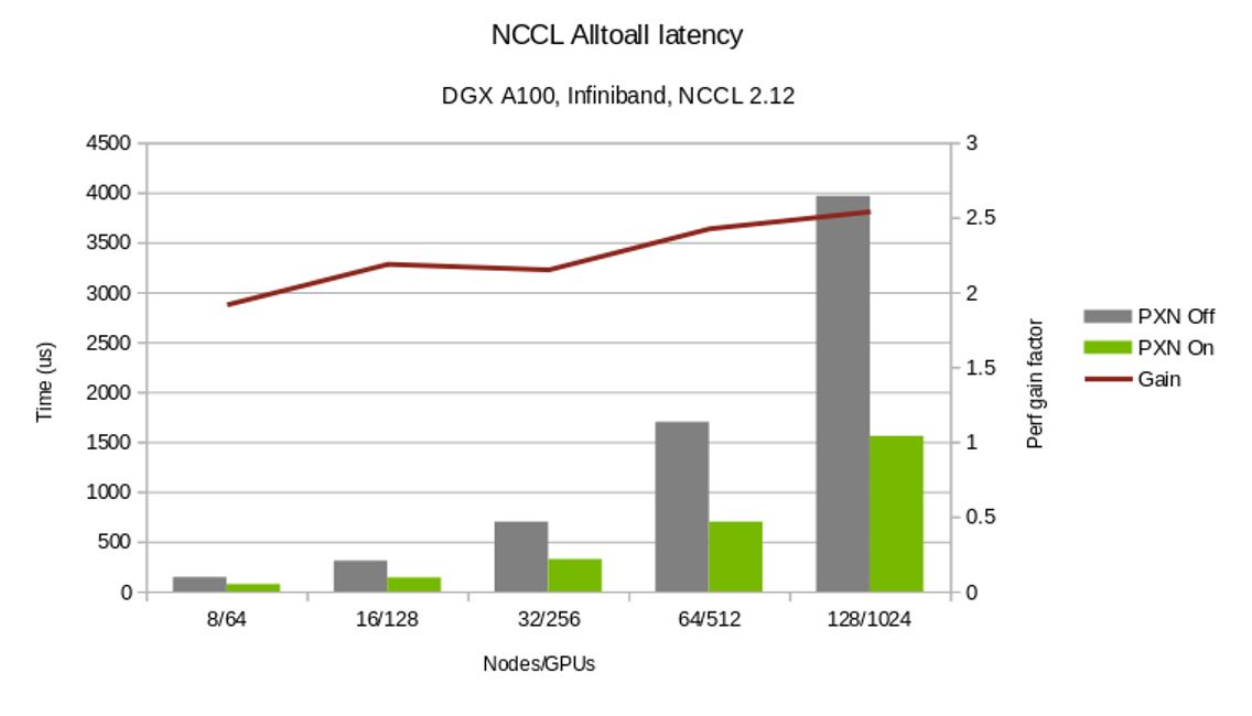
The NCCL 2.12 release significantly improves all2all communication collective performance, with the PXN feature.

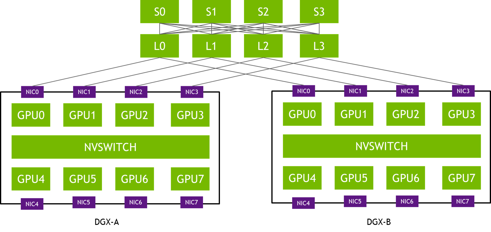
Collective communications are a performance-critical ingredient of modern distributed AI training workloads such as recommender systems and natural language processing.

NVIDIA Collective Communication Library (NCCL), a Magnum IO Library, implements GPU-accelerated collective operations:

• all-gather
• all-reduce
• broadcast
• reduce
• reduce-scatter
• point-to-point send and receive

NCCL is topology-aware and is optimized to achieve high bandwidth and low latency over PCIe, NVLink, Ethernet, and InfiniBand interconnect. NCCL GCP plugin and NCCL AWS plugin enable high-performance NCCL operations in popular cloud environments with custom network connectivity.

NCCL releases have been relentlessly focusing on improving collective communication performance. This post focuses on the improvements that come with the NCCL 2.12 release.

Combining NVLink and network communication

The new feature introduced in NCCL 2.12 is called PXN, as PCI × NVLink, as it enables a GPU to communicate with a NIC on the node through NVLink and then PCI. This is instead of going through the CPU using QPI or other inter-CPU protocols, which would not be able to deliver full bandwidth. That way, even though each GPU still tries to use its local NIC as much as possible, it can reach other NICs if required.

Instead of preparing a buffer on its local memory for the local NIC to send, the GPU prepares a buffer on an intermediate GPU, writing to it through NVLink. It then notifies the CPU proxy managing that NIC that the data is ready, instead of notifying its own CPU proxy. The GPU-CPU synchronization might be a little slower because it may have to cross CPU sockets, but the data itself only uses NVLink and PCI switches, guaranteeing maximum bandwidth.

In the topology in Figure 1, NIC-0 from each DGX system is connected to the same leaf switch (L0), NIC-1s are connected to the same leaf switch (L1), and so on. Such a design is often called rail-optimized. Rail-optimized network topology helps maximize all-reduce performance while minimizing network interference between flows. It can also reduce the cost of the network by having lighter connections between rails.

PXN leverages NVIDIA NVSwitch connectivity between GPUs within the node to first move data on a GPU on the same rail as the destination, then send it to the destination without crossing rails. That enables message aggregation and network traffic optimization.

Before NCCL 2.12, the message in Figure X would have traversed through three hops of network switches (L0, S1, and L3), potentially causing contention and being slowed down by other traffic. The messages passed between the same pair of NICs are aggregated to maximize effective message rate and network bandwidth.

Message aggregation

With PXN, all GPUs on a given node move their data onto a single GPU for a given destination. This enables the network layer to aggregate messages, by implementing a new multireceive function. The function enables the remote CPU proxy to send all messages as one as soon as they are all ready.

For example, if a GPU on a node is performing an all2all operation and is to receive data from all eight GPUs from a remote node, NCCL calls a multireceive with eight buffers and sizes. On the sender side, the network layer can then wait until all eight sends are ready, then send all eight messages at one time, which can have a significant effect on the message rate.

Another aspect of message aggregation is that connections are now shared between all GPUs of a node for a given destination. This means fewer connections to establish. It can also affect the routing efficiency, if the routing algorithm was relying on having a lot of different connections to get good entropy.

PXN improves all2all performance

Figure 3 shows that all2all entails communication from each process to every other process. In other words, the number of messages exchanged as part of an all2all operation in an N-GPU cluster is $latex  O(N^{2})$.

The messages exchanged between the GPUs are distinct and can’t be optimized using algorithms such as tree/ring (used for allreduce). When you run billion+ parameter models across 100s of GPUs, the number of messages can trigger congestion, create network hotspots, and adversely affect performance.

As discussed earlier, PXN combines NVLink and PCI communications to reduce traffic flow through the second-tier spine switches and optimizes network traffic. It also improves message rates by aggregating up to eight messages into one. Both improvements significantly improve all2all performance. 

all-reduce on 1:1 GPU:NIC topologies

Another problem that PXN solves is the case of topologies where there is a single GPU close to each NIC. The ring algorithm requires two GPUs to be close to each NIC. Data must go from the network to a first GPU, go around all GPUs through NVLink, and then exit from the last GPU onto the network. The first and last GPUs must both be close to the NIC. The first GPU must be able to receive from the network efficiently, and the last GPU must be able to send through the network efficiently. If only one GPU is close to a given NIC, then you cannot close the ring and must send data through the CPU, which can heavily affect performance.

With PXN, as long as the last GPU can access the first GPU through NVLink, it can move its data to the first GPU. The data is sent from there to the NIC, keeping all transfers local to PCI switches.

This case is not only relevant for PCI topologies featuring one GPU and one NIC per PCI switch but can also happen on other topologies when an NCCL communicator only includes a subset of GPUs. Consider a node with 8xGPUs interconnected with an NVLink hypercube mesh. 

Figure 5 shows a ring that can be formed by leveraging the high-bandwidth NVLink connections that are available in the topology when the communicator includes all the 8xGPUs in the system. This is possible as both GPU0 and GPU1 share access to the same local NIC.

The communicator can just include a subset of the GPUs. For example, it can just include GPUs 0, 2, 4, and 6. In that case, creating rings is impossible without crossing rails: rings entering the node from GPU 0 would have to exit from GPUs 2, 4, or 6, which do not have direct access to the local NICs of GPUs 0 (NICs 0 and 1).

On the other hand, PXN enables rings to be formed as GPU 2 could move data back to GPU 0 before going through NIC 0/1.

This case is common with model parallelism, depending on how the model is split. If for example a model is split between GPUs 0-3, then another model runs on GPUs 4-7. That means GPU 0 and 4 take care of the same part of the model, and an NCCL communicator is created with all GPUs 0 and 4 on all nodes, to perform all-reduce operations for the corresponding layers. Those communicators can’t perform all-reduce operations efficiently without PXN.

The only way to have efficient model parallelism so far was to split the model on GPUs 0, 2, 4, 6 and 1, 3, 5, 7 so that NCCL subcommunicators would include GPUs [0,1], [2,3], [4,5] and [6,7] instead of [0,4], [1,5], [2,6], and [3,7]. The new PXN feature gives you more flexibility and eases the use of model parallelism.

Figure 6 contrasts the time to complete alltoall collective operations with and without the PXN. In addition, PXN enables a more flexible choice of GPUs for all-reduce operations. 

Summary

The NCCL 2.12 release significantly improves all2all communication collective performance. Download the latest NCCL release and experience the improved performance firsthand.

For more information see the following resources:

• NCCL product page
• NCCL: High-Speed Inter-GPU Communication for Large-Scale Training GTC session
• Massively Scale Your Deep Learning Training with NCCL 2.4

submitted by /u/quinseptopol
[visit reddit] [comments]

submitted by /u/Term_Grecos
[visit reddit] [comments]