I would like to share my project and show you how to apply tinyML approach to detect broken tooth conditions in the gearbox based upon recorded vibration data.
I used Raspberry Pi Pico, Arduino IDE, Neuton Tiny ML software I will give an answer to such a questions as:
Is it possible to make an AI-driven system that predicts gearbox failure on a simple $4 MCU? How to automatically build a compact model that does not require any additional compression? Can a non-data scientist implement such projects successfully?
Introduction and Business Constraint
In industry (e.g., wind power, automotive), gearboxes often operate under random speed variations. A condition monitoring system is expected to detect faults, broken tooth conditions and assess their severity using vibration signals collected under different speed profiles.
Modern cars have hundreds of thousands of details and systems where it is necessary to predict breakdowns, control the state of temperature, pressure, etc.As such, in the automotive industry, it is critically important to create and embed TinyML models that can perform right on the sensors and open up a set of technological advantages, such as:
Internet independence
No waste of energy and money on data transfer
Advanced privacy and security
In my experiment I want to show how to easily create such a technology prototype to popularize the TinyML approach and use its incredible capabilities for the automotive industry.
Neuton TinyML:Neuton**,** I selected this solution since it is free to use and automatically creates tiny machine learning models deployable even on 8-bit MCUs. According to Neuton developers, you can create a compact model in one iteration without compression.
Raspberry Pi Pico: The chip employs two ARM Cortex-M0 + cores, 133 megahertz, which are also paired with 256 kilobytes of RAM when mounted on the chip. The device supports up to 16 megabytes of off-chip flash storage, has a DMA controller, and includes two UARTs and two SPIs, as well as two I2C and one USB 1.1 controller. The device received 16 PWM channels and 30 GPIO needles, four of which are suitable for analog data input. And with a net $4 price tag.
The goal of this tutorial is to demonstrate how you can easily build a compact ML model to solve a multi-class classification task to detect broken tooth conditions in the gearbox.
Dataset Description
Gearbox Fault Diagnosis Dataset includes the vibration dataset recorded by using SpectraQuest’s Gearbox Fault Diagnostics Simulator.
Dataset has been recorded using 4 vibration sensors placed in four different directions and under variation of load from ‘0’ to ’90’ percent. Two different scenarios are included:1) Healthy condition 2) Broken tooth condition
There are 20 files in total, 10 for a healthy gearbox and 10 for a broken one. Each file corresponds to a given load from 0% to 90% in steps of 10%. You can find this dataset through the link: https://www.kaggle.com/datasets/brjapon/gearbox-fault-diagnosis
The experiment will be conducted on a $4 MCU, with no cloud computing carbon footprints 🙂
Step 1: Model training
For model training, I’ll use the free of charge platform, Neuton TinyML. Once the solution is created, proceed to the dataset uploading (keep in mind that the currently supported format is CSV only).
Number of coefficients = 397, File Size for Embedding = 2.52 Kb. That’s super cool! It is a really small model!Upon the model training completion, click on the Prediction tab, and then click on the Download button next to Model for Embedding to download the model library file that we are going to use for our device.
Step 2: Embedding on Raspberry Pico
Once you have downloaded the model files, it’s time to add our custom functions and actions. I am using Arduino IDE to program Raspberry Pico.
Note: Since we are going to make classification on the test dataset, we will use the CSV utility provided by Neuton to run inference on the data sent to the MCU via USB.
I tried to build the same model with TensorFlow and TensorFlow Lite as well. My model built with Neuton TinyML turned out to be 4.3% better in terms of Accuracy and 15.3 times smaller in terms of model size than the one built with TF Lite. Speaking of the number of coefficients, TensorFlow’s model has, 9, 330 coefficients, while Neuton’s model has only 397 coefficients (which is 23.5 times smaller than TF!).
The resultant model footprint and inference time are as follows:
Autonomous vehicle development and validation require the ability to replicate real-world scenarios in simulation. At GTC, NVIDIA founder and CEO Jensen Huang showcased new AI-based tools for NVIDIA DRIVE Sim that accurately reconstruct and modify actual driving scenarios. These tools are enabled by breakthroughs from NVIDIA Research that leverage technologies such as NVIDIA Omniverse platform Read article >
This week at GTC, we’re celebrating – celebrating the amazing and impactful work that developers and startups are doing around the world. Nowhere is that more apparent than among the members of our global NVIDIA Inception program, designed to nurture cutting-edge startups who are revolutionizing industries. The program is free for startups of all sizes Read article >
Warp is a Python API framework for writing GPU graphics and simulation code, especially within Omniverse.
Typically, real-time physics simulation code is written in low-level CUDA C++ for maximum performance. In this post, we introduce NVIDIA Warp, a new Python framework that makes it easy to write differentiable graphics and simulation GPU code in Python. Warp provides the building blocks needed to write high-performance simulation code, but with the productivity of working in an interpreted language like Python.
By the end of this post, you learn how to use Warp to author CUDA kernels in your Python environment and make use of some of the built-in high-level functionality that makes it easy to write complex physics simulations, such as an ocean simulation (Figure 1).
Figure 1. Ocean simulation in Omniverse using Warp
Installation
Warp is available as an open-source library from GitHub. When the repository has been cloned, you can install it using your local package manager. For pip, use the following command:
pip install warp
Initialization
After importing, you must explicitly initialize Warp:
import warp as wp
wp.init()
Launching kernels
Warp uses the concept of Python decorators to mark functions that can be executed on the GPU. For example, you could write a simple semi-implicit particle integration scheme as follows:
Because Warp is strongly typed, you should provide type hints to kernel arguments. To launch a kernel, use the following syntax:
    wp.launch(kernel=simple_kernel, # kernel to launch
              dim=1024,             # number of threads
              inputs=[a, b, c],     # parameters
              device="cuda")        # execution device
Unlike tensor-based frameworks such as NumPy, Warp uses a kernel-based programming model. Kernel-based programming more closely matches the underlying GPU execution model. It is often a more natural way to express simulation code that requires fine-grained conditional logic and memory operations. However, Warp exposes this thread-centric model of programming in an easy-to-use way that does not require low-level knowledge of GPU architecture.
Compilation model
Launching a kernel triggers a just-in-time (JIT) compilation pipeline that automatically generates C++/CUDA kernel code from Python function definitions.
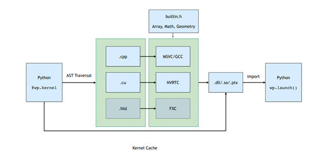
All kernels belonging to a Python module are runtime compiled into dynamic libraries and PTX. Figure 2. shows the compilation pipeline, which involves traversing the function AST and converting this to straight-line CUDA code that is then compiled and loaded back into the Python process.
Figure 2. Compilation pipeline for Warp kernels
The result of this JIT compilation is cached. If the input kernel source is unchanged, then the precompiled binaries are loaded in a low-overhead fashion.
Memory model
Memory allocations in Warp are exposed through the warp.array type. Arrays wrap an underlying memory allocation that may live in either host (CPU), or device (GPU) memory. Unlike tensor frameworks, arrays in Warp are strongly typed and store a linear sequence of built-in structures (vec3, matrix33, quat, and so on).
You can construct arrays from Python lists or NumPy arrays, or initialized, using a similar syntax to NumPy and PyTorch:
# allocate an uninitizalized array of vec3s
    v = wp.empty(length=n, dtype=wp.vec3, device="cuda")

    # allocate a zero-initialized array of quaternions
    q = wp.zeros(length=n, dtype=wp.quat, device="cuda")

    # allocate and initialize an array from a numpy array
    # will be automatically transferred to the specified device
    v = wp.from_numpy(array, dtype=wp.vec3, device="cuda")
Warp supports the __array_interface__, and __cuda_array_interface__ protocols, which allow zero-copy data views between tensor-based frameworks. For example, to convert data to NumPy use the following command:
# automatically bring data from device back to host
    view = device_array.numpy()
Features
Warp includes several higher-level data structures that make implementing simulation and geometry processing algorithms easier.
Meshes
Triangle meshes are ubiquitous in simulation and computer graphics. Warp provides a built-in type for managing mesh data that provide support for geometric queries, such as closest point, ray-cast, and overlap checks.
The following example shows how to use Warp to compute the closest point on a mesh to an array of input positions. This type of computation is the building block for many algorithms in collision detection (Figure 3). Warp’s mesh queries make it simple to implement such methods.
Figure 3. An example of collision detection against a complex object that uses closest-point mesh queries to test for contact between particles and the underlying object
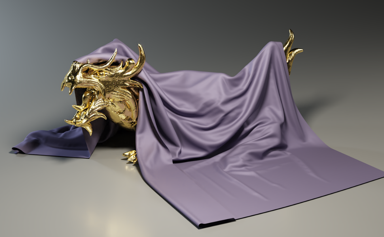
Sparse volumes are incredibly useful for representing grid data over large domains, such as signed distance fields (SDFs) for complex objects or velocities for large-scale fluid flow. Warp includes support for sparse volumes defined using the NanoVDB standard. Construct volumes using standard OpenVDB tools such as Blender, Houdini, or Maya, and then sample inside Warp kernels.
You can create volumes directly from binary grid files on disk or in-memory, and then sample them using the volumes API:
wp.volume_sample_world(vol, xyz, mode)  # world space sample using interpolation mode
wp.volume_sample_local(vol, uvw, mode)  # volume space sample using interpolation mode
wp.volume_lookup(vol, ijk)              # direct voxel lookup
wp.volume_transform(vol, xyz)           # map point from voxel space to world space
wp.volume_transform_inv(vol, xyz)       # map point from world space to volume space
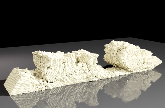
Figure 4. A particle simulation where the rock formation is represented as a sparse NanoVDB level set
Using volume queries, you can efficiently collide against complex objects with minimal memory overhead.
Hash grids
Many particle-based simulation methods, such as the discrete element method (DEM) or smoothed particle hydrodynamics (SPH), involve iterating over spatial neighbors to compute force interactions. Hash grids are a well-established data structure to accelerate these nearest neighbor queries and are particularly well suited to the GPU.
Hash grids are constructed from point sets as follows:
When hash grids are created, you can query them directly from within user kernel code as shown in the following example, which computes the sum of all neighbor particle positions:
@wp.kernel
def sum(grid : wp.uint64,
points: wp.array(dtype=wp.vec3),
output: wp.array(dtype=wp.vec3),
radius: float):
tid = wp.tid()
# query point
p = points[tid]
# create grid query around point
query = wp.hash_grid_query(grid, p, radius)
index = int(0)
sum = wp.vec3()
while(wp.hash_grid_query_next(query, index)):
neighbor = points[index]
# compute distance to neighbor point
dist = wp.length(p-neighbor)
if (dist
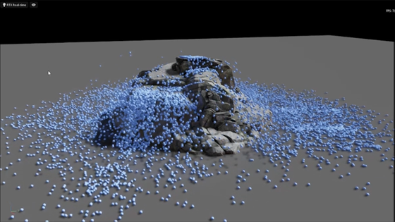
Figure 5 shows an example of a DEM granular material simulation for a cohesive material. Using the built-in hash-grid data structure allows you to write such a simulation in fewer than 200 lines of Python and runs at interactive rates for more than 100K particles.
Figure 5. An example of a DEM granular material simulation
Using the Warp hash-grid data allows you to easily evaluate the pairwise force interactions between neighboring particles.
Differentiability
Tensor-based frameworks, such as PyTorch and JAX, provide gradients of tensor computations and are well-suited for applications like ML training.
A unique feature of Warp is the ability to generate forward and backward versions of kernel code. This makes it easy to write differentiable simulations that can propagate gradients as part of a larger training pipeline. A common scenario is to use traditional ML frameworks for network layers, and Warp to implement simulation layers allowing for end-to-end differentiability.
When gradients are required, you should create arrays with requires_grad=True. For example, the warp.Tape class can record kernel launches and replay them to compute the gradient of a scalar loss function with respect to the kernel inputs:
After the backward pass has completed, the gradients with respect to the inputs are available through a mapping in the Tape object:
# gradient of loss with respect to input a
print(tape.gradients[a])
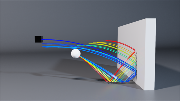
Figure 6. A trajectory optimization example where the initial velocity of the ball is optimized to hit the black target. Each line shows the result of one iteration of an LBFGS optimization step.
Summary
In this post, we presented NVIDIA Warp, a Python framework that makes it easy to write differentiable simulation code for the GPU. We encourage you to download the Warp preview release, share results, and give us feedback.
For more information, see the following resources:
Learn how servers can be built to deliver immersive workloads and take advantage of compute power to combine streaming XR applications with AI and other computing functions.
The current distribution of extended reality (XR) experiences is limited to desktop setups and local workstations, which contain the high-end GPUs necessary to meet computing requirements. For XR solutions to scale past their currently limited user base and support higher-end functionality such as AI services integration and on-demand collaboration, we need a purpose-built platform.
NVIDIA Project Aurora is a hardware and software platform that simplifies the deployment of enterprise XR applications onto corporate on-premises networks. This platform is also designed to support the integration of AI services within XR workloads.
Project Aurora leverages the XR streaming backbone of NVIDIA CloudXR and NVIDIA RTX Virtual Workstation (RTX vWS), bringing the horsepower of NVIDIA RTX A6000 and NVIDIA A40 to the edge to stream rich, real-time graphics from a machine room over a private 5G network.
Opportunities ahead
For XR developers, Project Aurora’s streamlined delivery of NVIDIA CloudXR streaming dramatically broadens the customer base from users tethered to high-power workstations to anyone with a simple headset or handheld device.
Users no longer need to leave their work areas to use a dedicated, attended, tethered “VR room” setup to experience high-power, high-quality immersion. Collaborators around the world, using their own separate local on-prem networks, can access and alter the same virtual environments at the same time.
Current use cases
Powerful XR use cases exist across multiple industries, allowing you to optimize workflows.
Medical professionals can explore immersive representations of anatomical models or even real patient data to train and work.
Manufacturing designers and engineers can shorten project lifecycles by leveraging digital twins of parts, assemblies, or entire manufacturing floors and plants.
Those same personnel can train in a virtual manufacturing environment without the need of physical resources or floor downtime.
Figure 1. Using a virtual experience through a reality headset
In collaboration with an ever-growing list of partners, NVIDIA has shown the value of moving these use cases into Project Aurora for virtualized distribution of XR over high performance networks.
BT and Ericsson
BT and Ericsson deployed a VR digital twin manufacturing solution on a 5G mobile private network using the world’s first 5G-enabled VR headset powered by the Qualcomm Snapdragon XR2 Platform. The experience runs on Masters of Pie’s Radical SDK, enabling cloud-based virtual reality within computer-aided design (CAD) software.
By seamlessly integrating the high-performance edge rendering provided by the Project Aurora platform, existing factory operations have benefited from high-fidelity VR experience that is available on the manufacturing floor.
EE 5G
Using augmented reality, The Green Planet AR Experience, powered by EE 5G, takes guests on an immersive journey into the secret kingdom of plants. Visitors travel through changing seasons on six digitally enhanced worlds, including rainforests, deserts, freshwater, and saltwater. The worlds are all powered by an Ericsson 5G standalone private network. Audiences engage and interact with the plant life by using a handheld mobile device, which acts as a window into the natural world.
The compute power of a handheld device on its own would not be nearly enough to render these volumetric models under normal conditions, but with Project Aurora, the experience is delivered seamlessly.
AT&T
AT&T recently teamed with Warner Bros., Ericsson, Qualcomm, Dreamscape, NVIDIA, and Wevr on an immersive, location-based VR experience, Chaos at Hogwarts. This proof-of-concept offers a peek into how Project Aurora combined with 5G can enhance future user-generated experiences.
By using the high-bandwidth and low-latency characteristics of 5G paired with Project Aurora’s XR infrastructure, we can change today’s architecture to one that is more comfortable for fans, more productive for creators, and more profitable for venue operators.
Project Aurora components
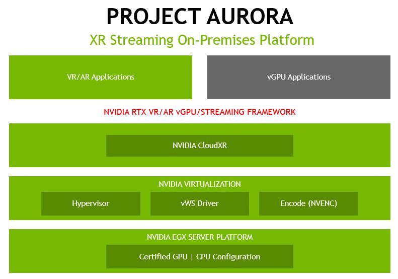
Project Aurora is an EGX certified server powered by a GPU/CPU configuration optimized for XR with a virtualization system using RTX vWS. The build is available through multiple OEMs (HPE, Dell) and supports multiple orchestration tools, including Linux KVM and VMWare vSphere.
NVIDIA CloudXR is layered on this virtualized workstation server to form the Project Aurora base platform. Although it is built specifically to stream XR applications, the Project Aurora server also supports any graphics-based workloads natively supported by RTX vWS.
Figure 2. Project Aurora architecture
The Project Aurora hardware and software stack is a scalable design built with the help of multiple partners. The base unit of an Aurora build consists of four highly optimized servers from Dell or HPE that support multiple NVIDIA A40 GPUs with RTX Virtual Workstation software and high-performance, low-latency NVIDIA networking components.
Network traffic has been carefully separated. It runs across multiple NVIDIA ConnectX network interface cards (NICs) and can be broken down into the following main areas:
Internal
External
Storage
These traffic flows are distributed across the three NICs to provide performance, security, and redundancy in each area in the event of any NIC failure. Project Aurora is designed with a “performance first” approach, and to scale from the base level to any size client deployment.
Project Aurora partners
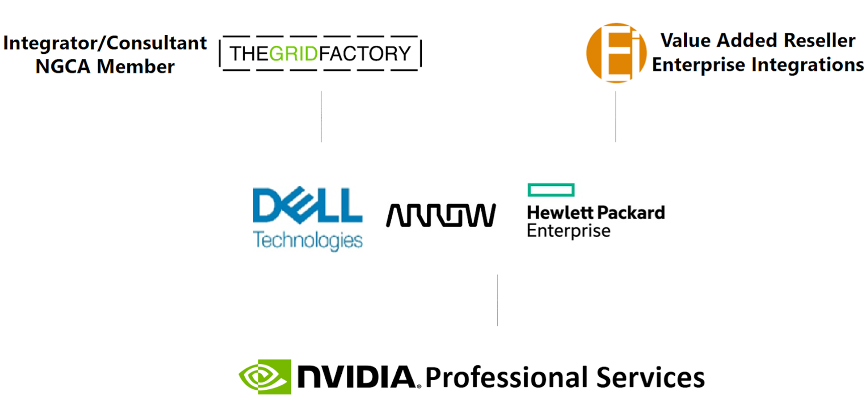
Project Aurora is more than just a scalable hardware and software platform. To make the Project Aurora platform easy for any IT crew to implement, NVIDIA has partnered with NVIDIA Partner Network (NPN) integration experts to assure that delivery and installation is simple, repeatable, and fully “white-glove.” Our sales distribution channel was built with the following partners:
The Grid Factory: Immersive technology integrator specializing in NVIDIA-based technologies, such as NVIDIA CloudXR, vGPU, Omniverse, and the EGX Server architecture.
Enterprise Integration: Value-added reseller coordinating between clients and various partners, including OEMs such as Dell and HPE and distributors such as Arrow.
NVIDIA Pro Services (NVPS): Delivers white-glove service to facilitate the standup of durable XR experiences.
Get started with Project Aurora
With the support of the NPN partners, to activate Project Aurora’s white-glove service, just contact one of our team members. The Project Aurora team works from application sizing and site survey through the ‘last-mile’ integration steps (authentication, profiling, server/network setup, tuning parameters, etc.) to achieve a successful XR distribution system.
Figure 3. Project Aurora partner network
Project Aurora customers are actively increasing towards hundreds, even thousands of users. If you are interested in learning more about Project Aurora or would like to get involved with our distribution channel to evaluate a new use case, contact Aurora_Outreach@nvidia.com.
This CUDA post examines the effectiveness of methods to hide memory latency using explicit prefetching.
NVIDIA GPUs have enormous compute power and typically must be fed data at high speed to deploy that power. That is possible, in principle, because GPUs also have high memory bandwidth, but sometimes they need your help to saturate that bandwidth.
In this post, we examine one specific method to accomplish that: prefetching. We explain the circumstances under which prefetching can be expected to work well, and how to find out whether these circumstances apply to your workload.
Context
NVIDIA GPUs derive their power from massive parallelism. Many warps of 32 threads can be placed on a streaming multiprocessor (SM), awaiting their turn to execute. When one warp is stalled for whatever reason, the warp scheduler switches to another with zero overhead, making sure the SM always has work to do.
On the high-performance NVIDIA Ampere Architecture A100 GPU, up to 64 active warps can share an SM, each with its own resources. On top of that, A100 has 108 SMs that can all execute warp instructions simultaneously.
Most instructions must operate on data, and that data almost always originates in the device memory (DRAM) attached to the GPU. One of the main reasons why even the abundance of warps on an SM can run out of work is because they are waiting for data to arrive from memory.
If this happens, and the bandwidth to memory is not fully utilized, it may be possible to reorganize the program to improve memory access and reduce warp stalls, which in turn makes the program complete faster. This is called latency hiding.
Prefetching
A technology commonly supported in hardware on CPUs is called prefetching. The CPU sees a stream of requests from memory arriving, figures out the pattern, and starts fetching data before it is actually needed. While that data travels to the execution units of the CPU, other instructions can be executed, effectively hiding the travel costs (memory latency).
Prefetching is a useful technique but expensive in terms of silicon area on the chip. These costs would be even higher, relatively speaking, on a GPU, which has many more execution units than the CPU. Instead, the GPU uses excess warps to hide memory latency. When that is not enough, you may employ prefetching in software. It follows the same principle as hardware-supported prefetching but requires explicit instructions to fetch the data.
To determine if this technique can help your program run faster, use a GPU profiling tool such as NVIDIA Nsight Compute to check the following:
Confirm that not all memory bandwidth is being used.
Confirm the main reason warps are blocked is Stall Long Scoreboard, which means that the SMs are waiting for data from DRAM.
Confirm that these stalls are concentrated in sizeable loops whose iterations do not depend on each other.
Unrolling
Consider the simplest possible optimization of such a loop, called unrolling. If the loop is short enough, you can tell the compiler to unroll it completely and the iterations are expanded explicitly. Because the iterations are independent, the compiler can issue all requests for data (“loads”) upfront, provided that it assigns distinct registers to each load.
These requests can be overlapped with each other, so that the whole set of loads experiences only a single memory latency, not the sum of all individual latencies. Even better, part of the single latency is hidden by the succession of load instructions itself. This is a near-optimal situation, but it may require a lot of registers to receive the results of the loads.
If the loop is too long, it could be unrolled partially. In that case, batches of iterations are expanded, and then you follow the same general strategy as before. Work on your part is minimal (but you may not be that lucky).
If the loop contains many other instructions whose operands need to be stored in registers, even just partial unrolling may not be an option. In that case, and after you have confirmed that the earlier conditions are satisfied, you must make some decisions based on further information.
Prefetching means bringing data closer to the SMs’ execution units. Registers are closest of all. If enough are available, which you can find out using the Nsight Compute occupancy view, you can prefetch directly into registers.
Consider the following loop, where array arr is stored in global memory (DRAM). It implicitly assumes that just a single, one-dimensional thread block is being used, which is not the case for the motivating application from which it was derived. However, it reduces code clutter and does not change the argument.
In all code examples in this post, uppercase variables are compile-time constants. BLOCKDIMX assumes the value of the predefined variable blockDim.x. For some purposes, it must be a constant known at compile time whereas for other purposes, it is useful for avoiding computations at run time.
for (i=threadIdx.x; i
}
Imagine that you have eight registers to spare for prefetching. This is a tuning parameter. The following code fetches four double-precision values occupying eight 4-byte registers at the start of each fourth iteration and uses them one by one, until the batch is depleted, at which time you fetch a new batch.
To keep track of the batches, introduce a counter (ctr) that increments with each successive iteration executed by a thread. For convenience, assume that the number of iterations per thread is divisible by 4.
double v0, v1, v2, v3;
for (i=threadIdx.x, ctr=0; i
}
Typically, the more values can be prefetched, the more effective the method is. While the preceding example is not complex, it is a little cumbersome. If the number of prefetched values (PDIST, or prefetch distance) changes, you have to add or delete lines of code.
It is easier to store the prefetched values in shared memory, because you can use array notation and vary the prefetch distance without any effort. However, shared memory is not as close to the execution units as registers. It requires an extra instruction to move the data from there into a register when it is ready for use. For convenience, we introduce macro vsmem to simplify indexing the array in shared memory:
#define vsmem(index)  v[index+PDIST*threadIdx.x]
__shared__ double v[PDIST* BLOCKDIMX];
for (i=threadIdx.x, ctr=0; i
}
Instead of prefetching in batches, you can also do a “rolling” prefetch. In that case, you fill the prefetch buffer before entering the main loop and subsequently prefetch exactly one value from memory during each loop iteration, to be used PDIST iterations later. The next example implements rolling prefetching, using array notation and shared memory.
__shared__ double v[PDIST* BLOCKDIMX];
for (k=0; k
}
Contrary to the batched method, the rolling prefetch does not suffer anymore memory latencies during the execution of the main loop for a sufficiently large prefetch distance. It also uses the same amount of shared memory or register resources, so it would appear to be preferred. However, a subtle issue may limit its effectiveness.
A synchronization within the loop—for example, syncthreads—constitutes a memory fence and forces the loading of arr to complete at that point within the same iteration, not PDIST iterations later. The fix is to use asynchronous loads into shared memory, the simplest version of which is explained in the Pipeline interface section of the CUDA programmer guide. These asynchronous loads do not need to complete at a synchronization point, but only when they are explicitly waited on.
Here’s the corresponding code:
#include
__shared__ double v[PDIST* BLOCKDIMX];
for (k=0; k
}
As each __pipeline_wait_prior instruction must be matched by a __pipeline_commit instruction, we put the latter inside the loop that prefills the prefetch buffer, before entering the main computational loop, to keep bookkeeping of matching instruction pairs simple.
Performance results
Figure 1 shows, for various prefetch distances, the performance improvement of a kernel taken from a financial application under the five algorithmic variations described earlier.
Batched prefetch into registers (scalar batched)
Batched prefetch into shared memory (smem batched)
Rolling prefetch into registers (scalar rolling)
Rolling prefetch into shared memory (smem rolling)
Rolling prefetch into shared memory using asynchronous memory copies (smem rolling async)
Figure 1. Kernel speedups for different prefetch strategies
Clearly, the rolling prefetching into shared memory with asynchronous memory copies gives good benefit, but it is uneven as the prefetch buffer size grows.
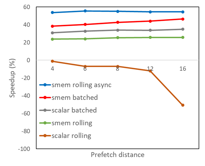
A closer inspection of the results, using Nsight Compute, shows that bank conflicts occur in shared memory, which cause a warp worth of asynchronous loads to be split into more successive memory requests than strictly necessary. The classical optimization approach of padding the array size in shared memory to avoid bad strides works in this case. The value of PADDING is chosen such that the sum of PDIST and PADDING equals a power of two plus 1. Apply it to all variations that use shared memory:
This leads to the improved shared memory results shown in Figure 2. A prefetch distance of just 6, combined with asynchronous memory copies in a rolling fashion, is sufficient to obtain optimal performance at almost 60% speedup over the original version of the code. We could actually have arrived at this performance improvement without resorting to padding by changing the indexing scheme of the array in shared memory, which is left as an exercise for the reader.
Figure 2. Kernel speedups for different prefetch strategies with shared memory padding
A variation of prefetching not yet discussed moves data from global memory to the L2 cache, which may be useful if space in shared memory is too small to hold all data eligible for prefetching. This type of prefetching is not directly accessible in CUDA and requires programming at the lower PTX level.
Summary
In this post, we showed you examples of localized changes to source code that may speed up memory accesses. These do not change the amount of data being moved from memory to the SMs, only their timing. You may be able to optimize more by rearranging memory accesses such that data is reused many times after it arrives on the SM.
NVIDIA Morpheus, now available for download, enables you to use AI to achieve up to 1000x improved performance.
Cybercrime worldwide is costing as much as the gross domestic product of countries like Mexico or Spain, hitting more than $1 trillion annually. And global trends point to it only getting worse.
Data centers face staggering increases in users, data, devices, and apps increasing the threat surface amid ever more sophisticated attack vectors.
Stop emerging threats
NVIDIA Morpheus enables cybersecurity developers and independent software vendors to build high-performance pipelines for security workflows with minimal development effort.
You can easily leverage the benefits of back pressure, reactive programming, and fibers to build cybersecurity solutions. The higher-level API enables you to program traditionally but gain the benefits of accelerated computing, allowing you to achieve orders of magnitude improvements in throughput. These optimizations don’t exist in any other streaming framework. Morpheus now enables building custom pipelines with Python and C++ abstraction layers.
You might typically have had to choose between writing something quickly in Python with minimal lines of code or writing something that doesn’t have the performance ceiling that Python does. With Morpheus, you get both.
You can write orders of magnitude less code and get an unbounded performance ceiling. This enables better results in less time, translating to cost savings and superior outcomes.
F5 malware detection
NVIDIA partner F5 used a Morpheus-based machine learning model for their malware detection use case. With its highly scalable, customizable, and accelerated data processing, training and inference capabilities, Morpheus enabled a 200x performance improvement to the F5 pipeline over their CPU-based implementation.
The Morpheus pipeline helps you quickly create highly performant code and workflows, which can incorporate innovative models, with minimal development friction. As a result, you extract better performance from GPUs, boosting processing of the logs required to find domain generation algorithms (DGAs).
Morpheus makes it easy to build and scale cybersecurity applications that harness adaptive pipelines supporting a wider range of model complexity than previously possible. Beyond just hardware acceleration, the programming model plays a critical role in performance. Morpheus uses reactive programming methods, which means that it can adapt and automatically redirect resources on the fly to any portion of the pipeline under pressure.
Figure 1. AI-Based, Real-Time Threat Detection at Scale
If part of the pipeline sees a dramatic increase in data, Morpheus can adapt and create additional paths for the data to continue processing. The depth of these buffers is monitored, and additional segments can be added as necessary. Just as easily, Morpheus removes these when they’re no longer necessary.
Using fibers, Morpheus can take work from other processes, if they’re being underused. You don’t have to spin up anything; just borrow the work available on those underused portions of the pipeline.
All this comes together to enable Morpheus to adapt intelligently to the high variability in cybersecurity data streams. It provides complete visibility into what’s happening on your network in real time and enables you to write sequential code that Morpheus scales out automatically.
With Morpheus, you can analyze up to 100% of your data in real time, for more accurate detection and faster remediation of threats as they occur. Morpheus also uses AI to adjust to threats and compensate on the fly.
Real-time fraud detection at scale
The Morpheus cybersecurity AI framework for developers is a first-of-its-kind offering for creating AI-accelerated, real-time fraud detection at massive scale.
Unleashing streaming graph neural networks (GNNs) for fraud detection, it unlocks capabilities that weren’t previously available to independent software vendors and security developers without hefty sums of labeled data.
GNNs achieve next-generation breakthroughs in fraud detection because they are uniquely designed to identify and analyze relationships between seemingly unconnected pieces of data to make predictions and do this at massive scale. It’s also why GNNs have historically been used for applications such as recommender systems and optimizing delivery routes for drivers.
Morpheus GNNs enable development on feature engineering for fraud detection with far less training data. With traditional approaches, experts identify pieces of data that are important, such as geolocation information and label them with their significance.
Because GNNs require less training data, you reduce the need for human expertise. You also enable the detection of threats that might not be otherwise recognized due to the amount of labeled training data required to train other models. Even with less data, you can improve the accuracy of fraud detection, which could potentially represent hundreds of millions of dollars to an organization.
Halt ransomware at the point of entry
Brazen global ransomware threats, like the high-profile shutdown of the Colonial Pipeline gas network, were an increased concern in 2021. Organizations are struggling to keep up with the volume and velocity of new threats. Costs of a data breach for an organization can run in the tens of millions per security breach and continue to rise.
The Morpheus AI application framework is built on NVIDIA RAPIDS and NVIDIA AI, together with NVIDIA GPUs. It enables the creation of powerful tools for implementing cybersecurity for this challenging era. When combined with the NVIDIA BlueField DPU accelerators and NVIDIA DOCA telemetry, this ushers in new standards for security development.
Figure 2. Morpheus architecture
Use cases for Morpheus include natural language processing (NLP) for phishing detection. Digital fingerprinting is another use case, as it analyzes the behavior of every human and machine across the enterprise to detect anomalies.
Join us at NVIDIA GTC to hear about how NVIDIA partners are integrating NVIDIA-accelerated AI with their cybersecurity solutions. NVIDIA Morpheus is open-source and available in April for download through GitHub and NGC.
For more information, see the following resources:
Interesting issue that I can’t quite wrap my head around.
We have a working Python project using Tensorflow to create and then use a model. This works great when we output the model as a directory, but if we output the model as an .h5 file, we run into the following error whenever we try to use the model:
ValueError: All `axis` values to be kept must have known shape. Got axis: (-1,), input shape: [None, None], with unknown axis at index: 1
Here is how we were and how we are currently saving the model:
# this technique works (saves model to a directory) tf.keras.models.save_model( dnn_model, filepath='./true_overall', overwrite=True, include_optimizer=True, save_format=None, signatures=None, options=None, save_traces=True ) #this saves the file, but throws an error when the file is used tf.keras.models.save_model( dnn_model, filepath='./true_overall.h5', overwrite=True, include_optimizer=True, save_format=None, signatures=None, options=None, save_traces=True )
This is how we’re importing the model for use:
dnn_model = tf.keras.models.load_model('./neural_network/true_overall.) #works dnn_model = tf.keras.models.load_model('./neural_network/true_overall.h5') #doesn't work
What would cause a model to work when saved as a directory but have issues when saved as an h5 file?
I am working on a project in which I am using layer wise relevance propagation to get the relevances of each input. But the output of LRP is in keras tensor. Is there any way to convert it to numpy array?
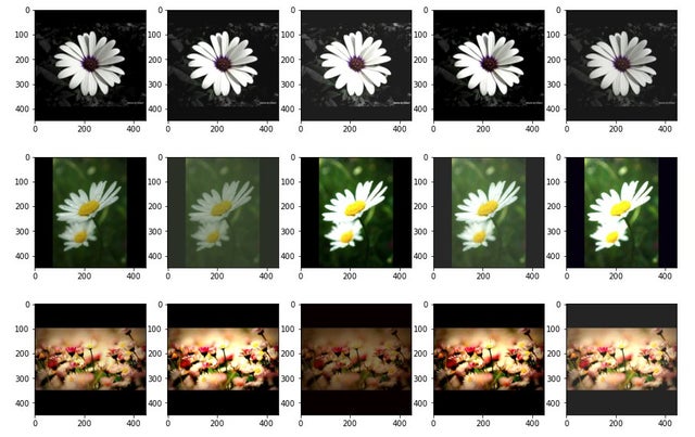
Hi there, I am a couple of weeks in with learning ML, and trying to get a decent image classifier. I have 60 or so labels, and only about 175-300 images each. I found that augmentation via flips and rotations suits the data and has helped bump up the accuracy a bit (maybe 7-10%).
The images have mostly white backgrounds, but some are not (greys, some darker) and this is not evenly distributed I think it was causing issues when making predictions from test photos: some incorrect labels came up frequently despite little visual similarity. I thought perhaps the background was involved as the darker background/shadows matched my photos. I figured adding contrast/brightness variation would nullify this behavior so I followed this here which adds a layer to randomize contrast and brightness to images in the training dataset. Snippet below:
With slight adjustments to contrast and brightness. I reviewed the output and it looks exactly how I wanted it, and I figured it would at least help, but it appears to cause a trainwreck! Does this make sense? Where should I look to improve on this?
As well, most tutorials focus on two labels, for 60 or so labels with 200-300 images each, in projects that deal with plants/nature/geology for example what is typically attainable for accuracy?


 Warp is a Python API framework for writing GPU graphics and simulation code, especially within Omniverse.
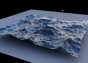
 Learn how servers can be built to deliver immersive workloads and take advantage of compute power to combine streaming XR applications with AI and other computing functions.
 This CUDA post examines the effectiveness of methods to hide memory latency using explicit prefetching.
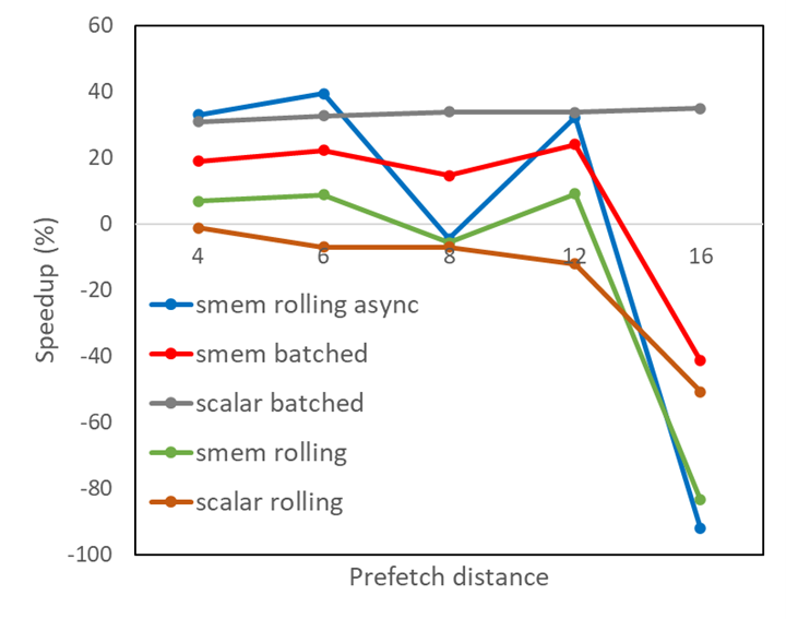
 NVIDIA Morpheus, now available for download, enables you to use AI to achieve up to 1000x improved performance.
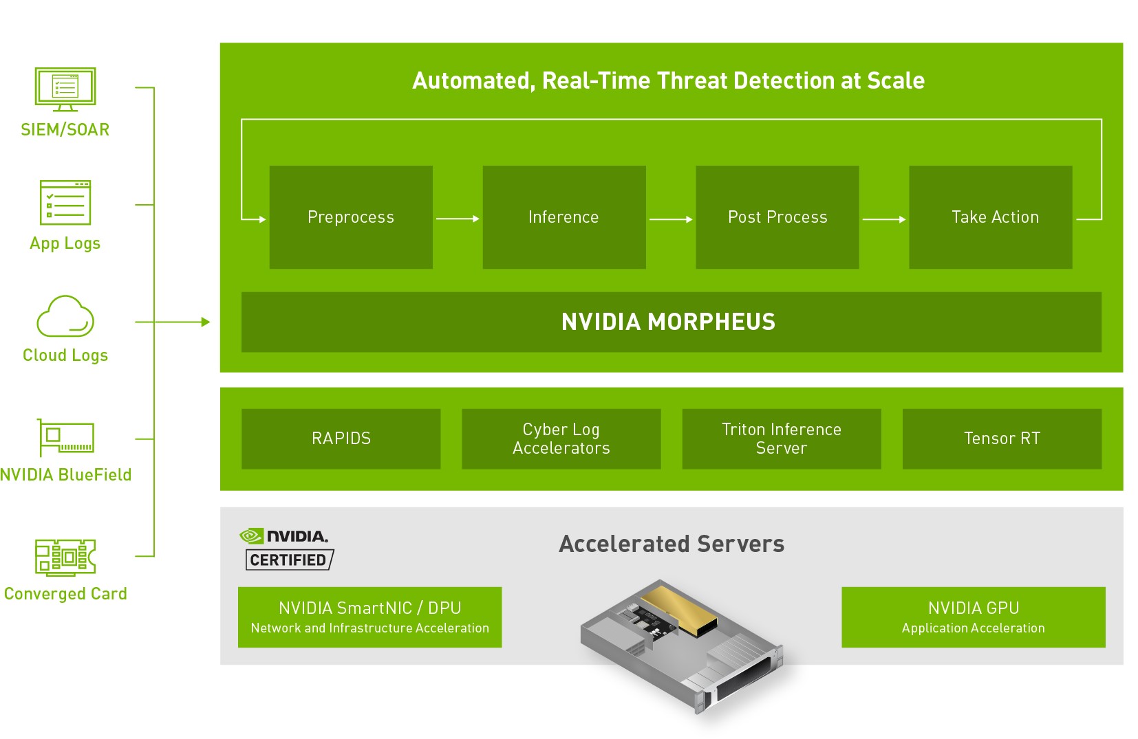
