SANTA CLARA, Calif., April 12, 2021 — GTC — NVIDIA today announced a range of eight new NVIDIA Ampere architecture GPUs for next-generation laptops, desktops and servers that make it possible…
It’s time to hail the new era of transportation. During his keynote at the GPU Technology Conference today, NVIDIA founder and CEO Jensen Huang outlined the broad ecosystem of companies developing next-generation robotaxis on NVIDIA DRIVE. These forward-looking manufacturers are set to transform the way we move with safer, more efficient vehicles for everyday mobility. Read article >
The post Top Robotaxi Companies Hail Rides on NVIDIA DRIVE appeared first on The Official NVIDIA Blog.
Kicking off NVIDIA’s GTC tech conference, NVIDIA CEO Jensen Huang weaves latest advancements in AI, automotive, robotics, 5G, real-time graphics, collaboration and data centers into a stunning vision of the future.
The post NVIDIA CEO Introduces Software, Silicon, Supercomputers ‘for the Da Vincis of Our Time’ appeared first on The Official NVIDIA Blog.
The electric vehicle revolution is about to reach the next level. Leading startups and EV brands have all announced plans to deliver intelligent vehicles to the mass market beginning in 2022. And these new, clean-energy fleets will achieve AI capabilities for greater safety and efficiency with the high-performance compute of NVIDIA DRIVE. The car industry Read article >
The post New Energy Vehicles Power Up with NVIDIA DRIVE appeared first on The Official NVIDIA Blog.
SANTA CLARA, Calif., April 12, 2021 (GLOBE NEWSWIRE) — NVIDIA today announced at its annual Investor Day that first quarter revenue for fiscal 2022 is tracking above its previously provided …
 Data plays a crucial role in creating intelligent applications. To create an efficient AI/ ML app, you must train machine learning models with high-quality, labeled datasets. Generating and labeling such data from scratch has been a critical bottleneck for enterprises. Many companies prefer a one-stop solution to support their AI/ML workflow from data generation, data … Continued
Data plays a crucial role in creating intelligent applications. To create an efficient AI/ ML app, you must train machine learning models with high-quality, labeled datasets. Generating and labeling such data from scratch has been a critical bottleneck for enterprises. Many companies prefer a one-stop solution to support their AI/ML workflow from data generation, data labeling, model training/fine-tuning, and deployment.
To fast track the end-to-end workflow for developers, NVIDIA has been working with several partners who focus on generating large, diverse, and high-quality labeled data. Their platforms can be seamlessly integrated with NVIDIA Transfer Learning Toolkit (TLT) and NeMo for training and fine-tuning models. These efficiently trained and optimized models can then be deployed with NVIDIA DeepStream or NVIDIA Jarvis to create reliable computer vision or conversational AI applications.
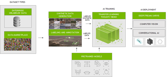
In this post, we outline the key challenges in data preparation and training. We also introduce how to integrate your data to fine-tune AI/ML models easily with our partner services.
Computer vision
Large amounts of labeled data are needed to train computer vision neural network models. They could be collected from the real world or synthesized through models. High-quality labeled data enables neural network models to contextualize the information and generate accurate results.
NVIDIA integrated with the platforms from the following partners to generate synthetic and label custom data in the formats compatible with TLT for training. TLT is a zero-coding transfer learning toolkit using purpose-built, pretrained models. Trained TLT models can be deployed using DeepStream SDK and achieve 10x speedup in development time.
AI Reverie and Sky Engine
Synthetic labeled data is becoming popular especially for computer vision tasks like object detection and image segmentation. Using the platforms from AI Reverie and Sky Engine, you can generate synthetic labeled data. AI Reverie offers a suite of synthetic data for model training and validation using 3D environments which exposes the neural network models to diverse scenarios that might be hard to find in data gleaned from the real world. Sky Engine uses ray-tracing image renderer techniques to generate labeled synthetic data in virtual environments that can be used with TLT for training.

Appen
With Appen, you can generate and label custom data. Appen uses APIs and human intelligence to generate labeled training data. Integrated with the NVIDIA Transfer Learning Toolkit, the Appen Data Annotation platform and services allow you to eliminate time-consuming annotations and create the right training data to train with TLT for your use cases.
Hasty, Labelbox, and Sama
Few provide straightforward tools for annotation. By simple clicks and selecting the region around the objects on the image, you can quickly generate the annotations. With Hasty, Sama, and Labelbox, you can label datasets in the formats compatible with TLT. TLT is a zero-coding transfer learning toolkit using purpose-built, pretrained models. Trained TLT models can be deployed using the DeepStream SDK and achieve 10x speedup in development time.
Hasty provides such tools like DEXTR and GrabCut to create labeled data. With DEXTR, you click on the north, south, east, and west of an object and a neural network looks for the mask. For GrabCut, you select the area where the object is and add or remove regions with markings to improve the results.
With Labelbox, you can upload the data for annotation and can easily export the annotated data using Python SDK to TLT for training purposes.
Sama follows a different labeling mechanism and therefore uses a pretrained object detection model (Figure 2) to perform inference. IT uses those annotations to further enhance the labels in generating accurate results.
All these tools are tightly coupled with TLT for training to develop production-quality vision models.
Conversational AI
A typical conversational AI application may be built with automatic speech recognition (ASR), natural language understanding (NLU), dialog management (DM) and text-to-speech (TTS) services. Conversational AI models are huge and require large amounts of data for training to recognize speech in noisy environments in different languages or accents, understand every nuance of language and generate human-like speech.
NVIDIA collaborates with DefinedCrowd, LabelStudio, and DataSaur. You can use their platforms to create large and labeled datasets that can then be directly introduced into NVIDIA NeMo for training or fine-tuning. NVIDIA NeMo is an open-source toolkit for developing state-of-the-art conversational AI models.
DefinedCrowd
The popular approach for data generation/labeling is crowdsourcing. DefinedCrowd leverages a global crowd of over 500,000 contributors to collect, annotate, and validate training data by dividing the project into a series of micro-tasks through the online platform Neevo. The data is then used to train conversational AI models in a variety of languages, accents, and domains. You can now quickly download the data using the DefinedCrowd APIs and convert them into NeMo acceptable format for training.
LabelStudio

Advancement of machine learning models make AI-assisted data annotation possible, which significantly reduces labeling cost. More and more vendors are integrating AI capability to augment the labeling process. NVIDIA collaborated with Heartex who maintains the open-source LabelStudio and performs AI-assisted data annotation for speech. With this tool, you can now label speech data that is compatible with NeMo (Figure 3). Heartex also integrates NeMo into their workflow so that you can choose the pretrained NeMo models for speech pre-annotation.
Datasaur
For text labeling, there are easy-to-use tools that come with predefined labels which allow you to quickly annotate the data. For more information about how to annotate your text data and run Datasaur with NeMo for training, see Datasaur x NVIDIA NeMo Integration (video).
Conclusion
NVIDIA has partnered with many industry-leading data generation and annotation providers to speed up computer vision and conversational AI application workflows. This collaboration enables you to quickly generate superior quality data that can be readily used with TLT and NeMo for training models, which can then be deployed on NVIDIA GPUs with DeepStream SDK and Jarvis.
For more information, see the following resources:
NVIDIA HPC SDK 21.3 Now Available
 The NVIDIA HPC SDK is a comprehensive suite of compilers, libraries, and tools enabling developers to program the entire HPC platform from the GPU foundation to the CPU, and through the interconnect.
Today, NVIDIA is announcing the availability of the HPC SDK version 21.3. This software can be downloaded now free of charge.
What’s New
- HPC-X toolkit, a comprehensive data communications package including MPI
- C++ stdpar support for multicore CPUs
- CUDA 11.2 Update 1
See the HPC SDK Release Notes for more information.
About the NVIDIA HPC SDK
The NVIDIA HPC SDK is a comprehensive suite of compilers, libraries, and tools enabling developers to program the entire HPC platform from the GPU foundation to the CPU, and through the interconnect. It is the only comprehensive, integrated SDK for programming accelerated computing systems.
The NVIDIA HPC SDK C++ and Fortran compilers are the first compilers to support automatic GPU acceleration of standard language constructs including C++17 parallel algorithms and Fortran intrinsics.
Learn more:
- GTC 2021: S31286 A Deep Dive into the Latest HPC Software — GTC is Free, Register Now
- GTC 2021: S31358 Inside NVC++
- NVIDIA HPC SDK Page
- NVIDIA HPC Compilers Page
- CUDA-X GPU-Accelerated Libraries Page
- Recent Developer Blog posts:
- 6 Ways to SAXPY
- Accelerating Standard C++ with GPUs Using stdpar
- Accelerating Fortran DO CONCURRENT with GPUs and the NVIDIA HPC SDK
- Bringing Tensor Cores to Standard Fortran
- Building and Deploying HPC Applications Using NVIDIA HPC SDK from the NVIDIA NGC Catalog
- Accelerating Python on GPUs with NVC++ and Cython
- HPC SDK Product Documentation
 Designing rich content and graphics for VR experiences means creating complex materials and high-resolution textures. But rendering all that content at VR resolutions and frame rates can be challenging, especially when rendering at the highest quality. You can address this challenge by using variable rate shading (VRS) to focus shader resources on certain parts of … Continued
Designing rich content and graphics for VR experiences means creating complex materials and high-resolution textures. But rendering all that content at VR resolutions and frame rates can be challenging, especially when rendering at the highest quality.
You can address this challenge by using variable rate shading (VRS) to focus shader resources on certain parts of an image—specifically, the parts that have the greatest impact for the scene, such as where the user is looking or the materials that need higher sampling rates.
However, because not all developers could integrate the full NVIDIA VRS API, NVIDIA developed Variable Rate Supersampling (VRSS), which increases the image quality in the center of the screen (fixed foveated rendering). VRSS is a zero-coding solution, so you do not need to add code to implement it. All the work is done through NVIDIA drivers, which makes it easy for users to experience VRSS in games and applications.
NVIDIA is now releasing VRSS 2, which now includes gaze-tracked, foveated rendering. The latest version further improves the perceived image quality by supersampling the region of the image where the user is looking. Applications that benefited from the original VRSS look even better with dynamic foveated rendering in VRSS 2.
New VR features
NVIDIA and Tobii collaborated to enhance VRSS with dynamic foveated rendering enabled by Tobii Spotlight, an eye-tracking technology specialized for foveation. This technology powers the NVIDIA driver with the latest eye-tracking information at minimal latency, which is used to control the supersampled region of the render frame. HPI’s upcoming Omnicept G2 HMD will be the first HMD on the market that takes advantage of this integration, as it uses both Tobii’s gaze-tracking technology and NVIDIA VRSS 2.
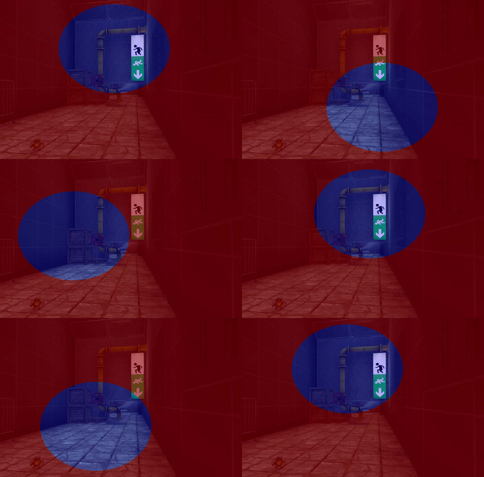
Accessing VRSS in the NVIDIA control panel
VRSS has two modes in the NVIDIA Control Panel: Adaptive and Always On.
Adaptive mode
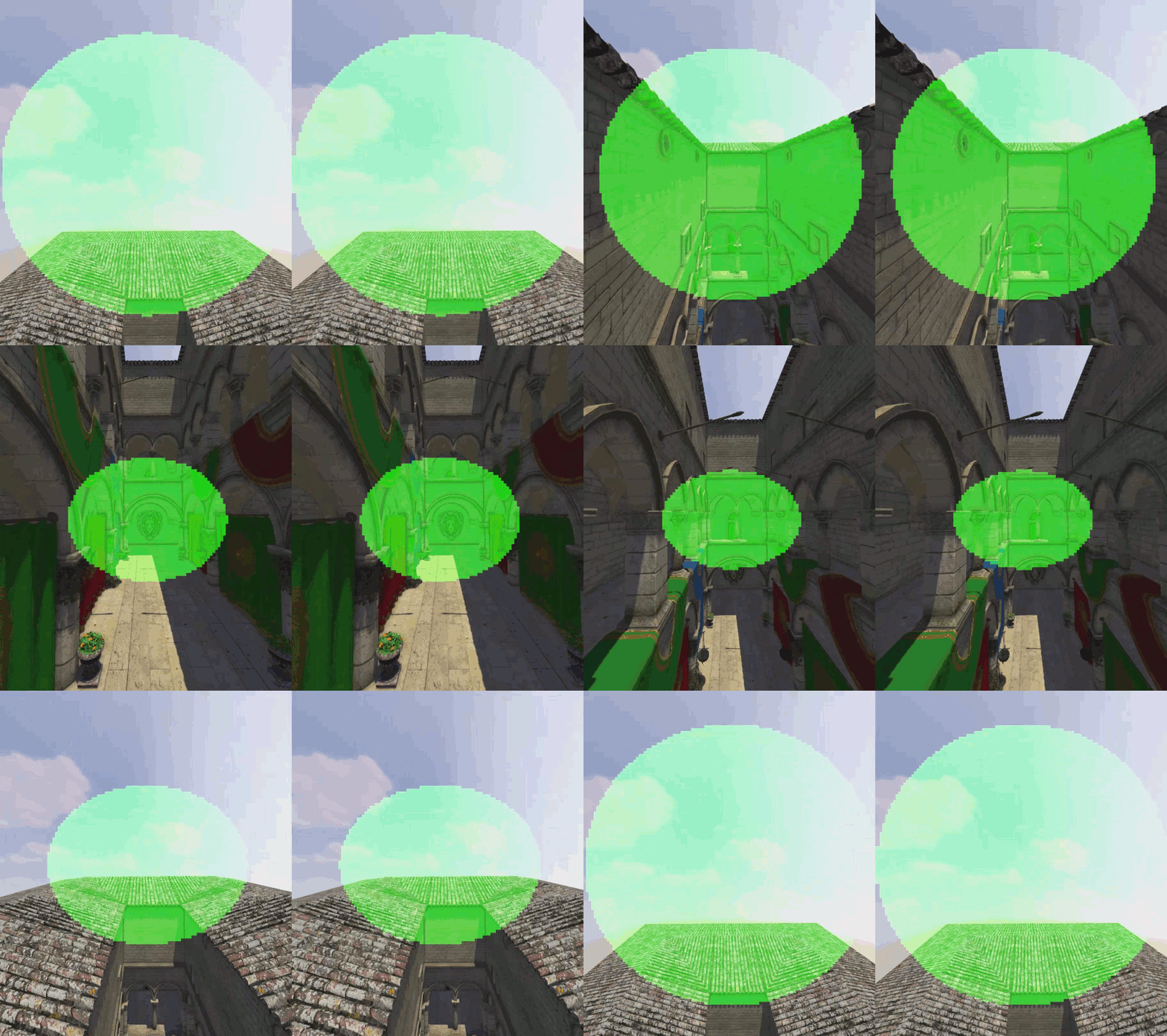
This mode takes performance limits into consideration and tries to maximize the size of the supersampling region without hindering the VR experience. The size of the foveated region grows and shrinks in proportion to the available GPU headroom.
Figure 4. Depicting the dynamic sizing of the foveated region in Adaptive mode. The supersampled region is depicted with a green mask. Supersampled region shrinks and grows based on the GPU load (scene complexity).
Always On mode
A fixed-size foveated region is always supersampled, providing maximum image quality improvements. The size of the foveated region is adequate to cover the central portion of the user’s field of view. This mode helps users perceive the maximum IQ gains possible for a given title using VRSS. However, this may also result in frame drops for applications that are performance intensive.
Under the hood
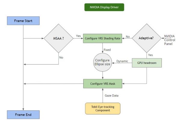
VRSS does not require any developer integration. The entire feature is implemented and handled inside the NVIDIA display driver, provided that the application is compatible and profiled by NVIDIA.
The NVIDIA display driver handles several pieces of functionality internally:
- Frame resources tracking—The driver keeps track of the resources encountered per frame and builds a heuristic model to flag a scenario where VRS could be invoked. Specifically, it notes the MSAA level to configure the VRS shading rate: the supersampling factor to be used at the center of the image. It provides render target parameters for configuring the VRS mask.
- Frame render monitoring—This involves measuring the rendering load across frames, the current frame rate of the application, the target frame rate based on the HMD refresh rate, and so on. This also computes the rendering stats required for the Adaptive mode.
- VRS enablement—As mentioned earlier, VRS gives you the ability to configure shading rate across the render surface. This is done with a shading rate mask and shading rate lookup table. For more information, see Turing Variable Rate Shading in VRWorks. The VRS infrastructure setup handles the configuration of the VRS mask and VRS shading rate table lookup. The VRS framework is configured based on the performance stats:
- VRS mask—The size of the central region mask is configured based on the available headroom.
- VRS shading rates—Configured based on the MSAA buffer sample count.
- Gaze data per frame—For VRSS 2, a component supplies the latest gaze data per frame. This involves a direct data transfer between the driver and the eye-tracking vendor platform. This data is used to configure the VRS foveation mask.
Developer guidance
For an application to take advantage of VRSS, you must submit your game or application to NVIDIA for VRSS validation. If approved, the game or application is added to an approved list within the NVIDIA driver.
Here are the benefits for a VRSS-supported game or application:
- The foveated region is now dynamic: Integration with Tobii Eye Tracking software.
- Zero coding: No developer integration required to work with game or application.
- Improved user experience: The user experiences VR content with added clarity.
- Ease of use: User controlled on/off supersampling in the NVIDIA Control Panel.
- Performance modes: Adaptive (fps priority) or Always On.
- No maintenance: Technology encapsulated at the driver level.
| Pavlov VR | L.A. Noire VR | Mercenary 2: Silicon Rising |
| Robo Recall | Eternity Warriors VR | Mercenary 2: Silicon Rising |
| Serious Sam VR: The Last Hope | Hot Dogs Horseshoes & Hand Grenades | Special Force VR: Infinity War |
| Talos Principle VR | Boneworks | Doctor Who: The Edge of time-VR |
| Battlewake | Lone Echo | VRChat |
| Job Simulator | Rec Room | PokerStars VR |
| Spiderman Homecoming VR | Rick & Morty Simulator: Virtual Rick-ality | Budget Cuts 2: Mission Insolvency |
| In Death | Skeet: VR Target Shooting | The Walking Dead: Saints & Sinners |
| Killing Floor: Incursion | SpiderMan far from home | Onward VR |
| Space Pirate Trainer | Sairento VR | Medal of Honor: Above and Beyond |
| The Soulkeeper VR | Raw Data | Sniper Elite VR |
Game and application compatibility
To make use of VRSS, applications must meet the following requirements:
- Turing architecture
- DirectX 11 VR applications
- Forward rendered with MSAA
- Eye-tracking software integrated with VRSS
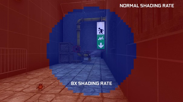
Supersampling needs an MSAA buffer. The level of supersampling is based on the underlying number of samples used in the MSAA buffer. The foveated region is shaded 2x for 2x MSAA, 4x supersampled for 4x MSAA, and so on. The maximum shading rate applied for supersampling is 8x. The higher the MSAA level, the greater the supersampling effect will be.
Content suitability
Content that benefits from supersampling benefits from VRSS as well. Supersampling not only mitigates aliasing but also brings out details in an image. The degree of quality improvement varies across content.
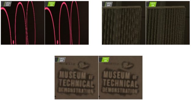
Supersampling shines when it encounters the following types of content:
- High-resolution textures
- High frequency materials
- Textures with alpha channels – fences, foliage, menu icons, text, and so on
Conversely, supersampling does not improve IQ for:
- Flat shaded geometry
- Textures and materials with low level of detail
Come onboard!
VRSS leverages VRS technology for selective supersampling and does not require application integration. VRSS is available in NVIDIA Driver R465, and applications are required to support DX11, forward rendering, and MSAA.
Submit your game and application to NVIDIA for VRSS consideration.
If you want finer-grained control of how VRS is applied, we recommend using the explicit programming APIs of VRWorks – Variable Rate Shading (VRS). Accessing the full power of VRS, you can implement a variety of shader sampling rate optimizations, including lens-matched shading, content-adaptive shading, and gaze-tracked shading.
 Magnum IO is the collection of IO technologies from NVIDIA and Mellanox that make up the IO subsystem of the modern data center and enable applications at scale. If you are trying to scale up your application to multiple GPUs, or scaling it out across multiple nodes, you are probably using some of the libraries … Continued
Magnum IO is the collection of IO technologies from NVIDIA and Mellanox that make up the IO subsystem of the modern data center and enable applications at scale. If you are trying to scale up your application to multiple GPUs, or scaling it out across multiple nodes, you are probably using some of the libraries in Magnum IO. NVIDIA is now publishing the Magnum IO Developer Environment 21.04 as an NGC container, containing a comprehensive set of tools to scale IO. This allows you to begin scaling your applications on a laptop, desktop, workstation, or in the cloud.
Magnum IO brings the ability to improve end-to-end wall clock time of IO bound applications. Imagine a workflow with three stages:
- ETL (extract, transform, load)
- Scaled-out compute
- Post-processing and output
The first-stage ETL jobs are dominated by reading large amounts of data into GPUs and can achieve optimal performance by using Magnum IO GPUDirect Storage (GDS) for directly copying data from storage into GPU memory. This also helps reduce the CPU utilization and improves overall data center utilization.
The second stage, which comprises a distributed communication GPU-to-GPU IO intense job, can benefit from optimizing communication with NCCL message-passing or NVSHMEM shared memory models, on low latency InfiniBand networks.
The final post-processing and output stages, as well as the checkpointing and temporary storage during the workflow, can again improve performance with GDS. Magnum IO management layers also enable monitoring, troubleshooting, and detecting anomalies of all the stages of the workflow.
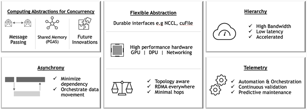
Scaling applications to run efficiently is often a complex and time-consuming task. We understand that the changes to code to adopt the Magnum IO technologies can be invasive, and any changes require development, debugging, testing, and benchmarking. Magnum IO libraries also work alongside the profilers, logging, and monitoring tools needed to observe what’s happening, locate bottlenecks, and address them. You should understand the performance tradeoffs of each stage of the computation and understand the relationships and between the hardware components in the system.
Magnum IO libraries provide APIs that manage the underlying hardware, allowing you to focus on the algorithmic aspects of your applications. The APIs are designed to be high-level so that they are easy to integrate with, but also to expose finer controls for when you start fine-tuning performance, after the behaviors and tradeoffs of the application running at scale are understood.
The high bandwidth and low latency offered by NVLink operating at 300GB/s, and InfiniBand in NVIDIA DGX A100 systems also opens new possibilities for algorithms. The NVLink bandwidth between GPUs now makes remote memory almost local. The total number of PCIe lanes from remote storage may exceed those from local storage. Magnum IO libraries on NVIDIA hardware allow algorithms to take full advantage of the GPU memory across all nodes, rather than sacrificing efficiency to avoid what was bottlenecking IO with high latencies in the past.

Magnum IO: GPU-to-GPU communications
Core to Magnum IO are libraries that allow GPUs to talk directly to each other over the fasted links available.
NCCL
The NVIDIA Collective Communications Library (NCCL, pronounced “nickel”) is a library providing inter-GPU communication primitives that are topology-aware and can be easily integrated into applications.
NCCL is smart about IO on systems with complex topology: systems with multiple CPUs, GPUs, PCI busses, and network interfaces. It can selectively use NVLink, Ethernet, and InfiniBand, using multiple links when possible. Consider using NCCL APIs whenever you plan your application or library to run on a mix of multi-GPU multi-node systems in a data center, cloud, or hybrid system. At runtime, NCCL determines the topology and optimizes layout and communication methods.
NVSHMEM
NVSHMEM creates a global address space for data that spans the memory of multiple GPUs and can be accessed with fine-grained GPU-initiated operations, CPU-initiated operations, and operations on CUDA streams.
In many HPC workflows, models and simulations are run that far exceed the size of a single GPU or node. NVSHMEM allows for a simpler asynchronous communication model in a shared address space that spans GPUs within or across nodes, with lower overheads, possibly resulting in stronger scaling compared to a traditional Message Passing Interface (MPI).
UCX
Unified Communication X (UCX) uses high-speed networks, including InfiniBand, for inter-node communication and shared memory mechanisms for efficient intra-node communication. If you need a standard CPU-driven MPI, PGAS OpenSHMEM libraries, and RPC, GPU-aware communication is layered on top of UCX.
UCX is appropriate when driving IO from the CPU, or when system memory is being shared. UCX enables offloading the IO operations to both host adapter (HCA) and switch, which reduces CPU load. UCX simplifies the portability of many peer-to-peer operations in MPI systems.
Magnum IO: Storage-to-GPU communications
Magnum IO also addresses the need to move data between GPUs and storage systems, both local and remote, with as little overhead as possible along the way.
GDS
NVIDIA GPUDirect Storage (GDS) enables a direct data path for Remote Direct Memory Access (RDMA) transfers between GPU memory and storage, which avoids a bounce buffer and management by the CPU. This direct path increases system bandwidth and decreases the latency and utilization load on the CPU.
-
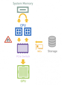
a) Without GDS -
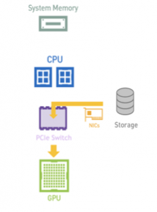
b) With GDS
GDS and the cuFile APIs should be used whenever data needs to move directly between storage and the GPU. With storage systems that support GDS, significant increases in performance on clients are observed when IO is a bottleneck. In cases where the storage system does not support GDS, IO transparently falls back to normal file reads and writes.
Moving the IO decode/encode from the CPU to GPU creates new opportunities for direct data transfers between storage and GPU memory which can benefit from GDS performance. An increasing number of data formats are supported in CUDA.
Magnum IO: Profiling and optimization
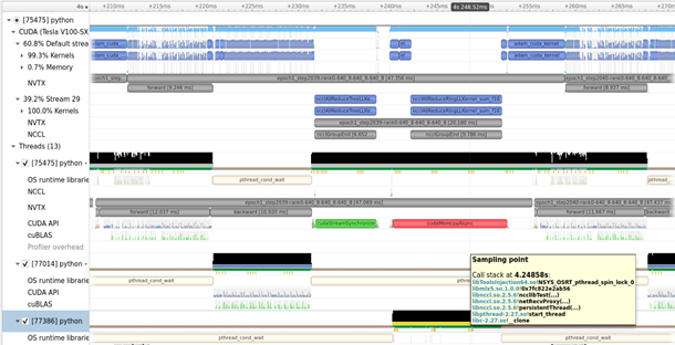
NVIDIA Nsight Systems lets you see what’s happening in the system and NVIDIA Cumulus NetQ allows you to analyze what’s happening on the NICs and switches. This is critical to finding some causes of bottlenecks in multi-node applications.
Nsight Systems
Nsight Systems is a low-overhead performance analysis tool designed to provide insights that you need to optimize your software. It provides everything that you would expect from a profiler for a GPU. Nsight Systems has a tight integration with many core CUDA libraries, giving you detailed information on what is happening.
Nsight Systems allows you to see exactly what’s happening on the system, what code is taking a long time, and when algorithms are waiting on GPU/CPU compute, or device IO. Nsight Systems is relevant to Magnum IO and included in the Magnum IO container for convenience, but its scope spans well outside of Magnum IO to monitoring compute that’s unrelated to IO.
NetQ
NetQ is a highly scalable, modern, network operations tool set that provides visibility, troubleshooting and lifecycle management of your open networks in real time. It enables network profiling functionality that can be used along with Nsight Systems or application logs to observe the network’s behavior while the application is running.
NetQ is part of Magnum IO itself, given its integral involvement in managing IO in addition to profiling it.
Getting started with the Magnum IO Developer Environment
We are launching the Magnum IO Developer Environment as a container hosted on NVIDIA NGC for GTC 21. A bare-metal installer for Ubuntu and RHEL may be coming soon. The container provides a sealed environment with the latest versions of the libraries compatible with each other. It makes it easy for you to begin optimizing your application’s IO. Installing and working with the container does not interfere with any existing system setup, which may have different versions of the components.
The Magnum IO components included in the 21.04 container are as follows:
- Ubuntu 20.04
- CUDA
- Nsight Systems CLI
- GDS
- GPUDirect RDMA
- GPUDirect P2P
- NCCL
- UCX
- NVSHMEM
The first step is to profile the application and find the bottlenecks, then evaluate which of the Magnum IO tools, libraries, or algorithm changes are appropriate for removing those bottlenecks and optimizing the application.
Download the developer environment today: Magnum IO SDK.
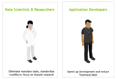
 In the field of medicine, advancements in artificial intelligence are constantly evolving. To keep up with the pace of innovation means adapting and providing the best experience to researchers, clinicians, and data scientists. NVIDIA Clara Train, an application framework for training medical imaging models, has undergone significant changes for its upcoming release at the beginning … Continued
In the field of medicine, advancements in artificial intelligence are constantly evolving. To keep up with the pace of innovation means adapting and providing the best experience to researchers, clinicians, and data scientists. NVIDIA Clara Train, an application framework for training medical imaging models, has undergone significant changes for its upcoming release at the beginning of May, with product enhancements for better AI model training.
In this post, I cover three new major features introduced in Clara Train 4.0:
- Upgrade of the underlying infrastructure of Clara Train based on MONAI.
- Expansion into digital pathology, with a training pipeline to help you get started.
- Update of the DeepGrow model to annotate organs effectively in 3D images.
The Clara Train Early Access program gives you access to all features: Sign up today!
First, Clara Train has updated its backend infrastructure to use MONAI, the Medical Open Network for AI. MONAI is an open-source, PyTorch-based framework that provides domain-optimized foundational capabilities for healthcare. This community-led library helps create reproducible experiments by reducing the need for duplication or re-implementation. Figure 2 shows the three layers that make up Clara Train.
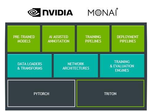
The top layer includes pretrained models that can be downloaded from the NGC catalog and which are now updated to work with MONAI. You can also continue to use all the features already in Clara Train, like AI-assisted annotation, federated learning, and training and deployment pipelines.
Specialized for training medical imaging models, the middle layer showcases MONAI components. These include data loaders and transforms, network architectures, and training and evaluation engines. MONAI aims to provide a comprehensive list of medical image–specific transformations and reference networks that provides flexibility and code readability.
The bottom layer highlights the two base frameworks that make up the foundation of MONAI and Clara Train. By being built on top of PyTorch, you receive all the benefits of using one of the most widely used machine learning frameworks, as well as the community support. For inference, Clara Train uses NVIDIA Triton, which simplifies the deployment of AI models and maximizes GPU utilization.
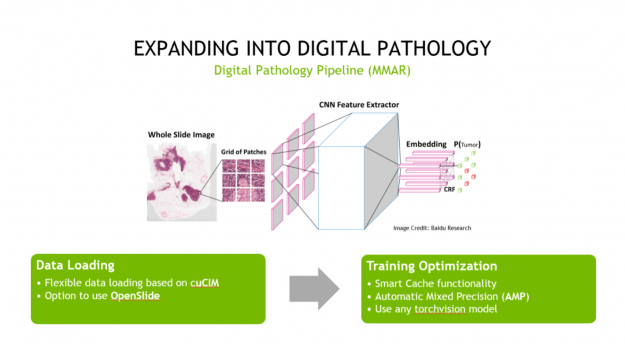
Second, Clara Train is expanding into digital pathology. And although digital pathology is an imaging workload, it differs significantly from radiology in its details and challenges. To help address these challenges, we’ve created a digital pathology pipeline.
This pipeline includes optimized data loading using cuCIM, which can tile large datasets on-demand and process them through a CUDA-enabled pipeline. It also includes training optimizations like Smart Cache, which re-uses a portion of data in memory at each epoch and produces a more efficient training workflow. Last, it includes a fully convolutional classification network that works with whole-slide images. All these features provide you with up to a 10x speedup in training, compared to other pathology pipelines.
To use cuCIM outside Clara Train, you can install it using pip by issuing the following command:
pip install cucim
We’ve also included a pretrained model that detects tumors in lymph nodes using whole-slide histopathology images. You can use this model to create your own digital pathology model.

Last, we’ve updated the DeepGrow model to work on 3D CT images. This updated model gives you the ability to segment an organ in 3D with only a few clicks across the organ. If you’re looking to create an organ-specific, DeepGrow 3D model, we’ve provided a pipeline to help you get started quickly.
Federated learning with homomorphic encryption
In Clara Train 4.0, we also added homomorphic encryption tools for federated learning. Homomorphic encryption allows you to compute data while the data is still encrypted.
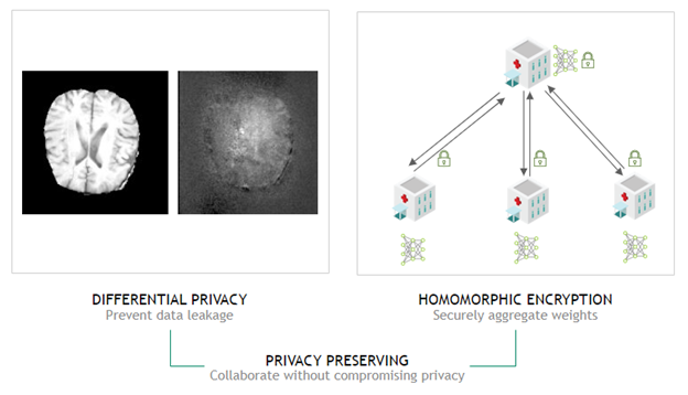
In Clara Train 3.1, all clients used certified SSL channels to communicate their local model updates with the server. The SSL certificates are needed to establish trusted communication channels and are provided through a third party that runs the provisioning tool and securely distributes them to the hospitals. This secures the communication to the server, but the server can still see the raw model (unencrypted) updates to do aggregation.
With Clara Train 4.0, the communication channels are still established using SSL certificates and the provisioning tool. However, each client optionally also receives additional keys to homomorphically encrypt their model updates before sending them to the server. The server doesn’t own a key and only sees the encrypted model updates. With homomorphic encryption, the server can aggregate these encrypted weights and then send the updated model back to the client. The clients can decrypt the model weights because they have the keys and can then continue with the next round of training.
Homomorphic encryption ensures that each client’s changes to the global model stays hidden by preventing the server from reverse-engineering the submitted weights and discovering any training data. This added security comes at a computational cost on the server. However, it can play an important role in healthcare in making sure that patient data stays secure at each hospital while still benefiting from using federated learning with other institutions.
Bring your own components to Clara Train
MONAI provides a lot of domain-specific functionality directly through their transformations, loss, and metric functions. These core components are independent modules and can be integrated into any PyTorch program. However, if you’re a researcher and developing state-of-the-art models, these components might not be sufficient.
When this is the case, you can include your own custom functions directly into Clara Train through the bring your own components (BYOC) functionality. By writing your components modularly and in Python, you can add them to the training configuration file.
Before getting started, you must define the Medical Model Archive (MMAR). In Clara Train, an MMAR defines a standard structure for organizing all artifacts produced during the model development life cycle and defining your training workflow. You modify these configuration files to add in your custom functions.
Here’s an example of how to do this by adding your own custom network architecture and loss function. First, start by defining these functions in their own Python file. For this example, assume that your custom functions are in a BYOC folder to make sure that you keep everything organized. This also allows you to see how the pathing works for calling out to your custom function from within the MMAR config file.
{
  "epochs": 10,
  "use_gpu": true,
  "multi_gpu": false,
  "amp": true,
  "determinism": {    },
  "train": {
    "loss": {

            },
    "optimizer": {    },
    "lr_scheduler": {    },
    "model": {

             },
    "pre_transforms": [    ],
    "dataset": {    },
    "dataloader": {    },
    "inferer": {    },
    "handlers": [    ],
    "post_transforms": [    ],
    "metrics": [    ],
    "trainer": {    }
  },
  "validate": {    }
}
For this post, we’re not including all the functions needed to create this network in the code examples. To see all the code required, see the complete example at NVIDIA/clara-train-examples in the BYOC Jupyter notebook.
The following code example defines your custom MyBasicUNet class, a UNet implementation with 1D, 2D, and 3D support, defined in a file labeled myNetworkArch.py:
from typing import Sequence, Union

import torch
import torch.nn as nn

from monai.networks.blocks import Convolution, UpSample
from monai.networks.layers.factories import Conv, Pool
from monai.utils import ensure_tuple_rep

class MyBasicUNet(nn.Module):
    def __init__(
        self,
        dimensions: int = 3,
        in_channels: int = 1,
        out_channels: int = 2,
        features: Sequence[int] = (32, 32, 64, 128, 256, 32),
        act: Union[str, tuple] = ("LeakyReLU", {"negative_slope": 0.1, "inplace": True}),
        norm: Union[str, tuple] = ("instance", {"affine": True}),
        dropout: Union[float, tuple] = 0.0,
        upsample: str = "deconv",
    ):
        super().__init__()
…
Next, you define the custom loss function that computes the average dice loss between two tensors. The following code example is a section of the MyDiceLoss class defined in a file labeled myLoss.py:
from typing import Callable, Optional, Union

import torch
from torch.nn.modules.loss import _Loss

from monai.networks import one_hot
from monai.utils import LossReduction, Weight

class MyDiceLoss(_Loss):
    def __init__(self,include_background: bool = True,to_onehot_y: bool = False,sigmoid: bool = False,softmax: bool = False,
        other_act: Optional[Callable] = None, squared_pred: bool = False, jaccard: bool = False,
        reduction: Union[LossReduction, str] = LossReduction.MEAN,smooth_nr: float = 1e-5,smooth_dr: float = 1e-5,batch: bool = False,
    ) -> None:
        super().__init__()
…
Now that you’ve defined the custom network and loss functions, here’s how to add them to the MMAR configuration. The configuration file for this run is labeled trn_BYOC_arch_loss.json, and you focus on two different sections of the JSON file.
First, add the custom network to the config by defining a train section and within that section a model field. This is where you add a reference to the custom model. When using an MMAR, you can also define arguments to pass to the function.
The following code example shows the train->model section of the config file:
"model": {
  "path": "BYOC.myNetworkArch.MyBasicUNet",
  "args": {
    "dimensions": 3,
    "in_channels": 1,
    "out_channels": 2,
    "features": [16, 32, 64, 128, 256, 16],
    "norm": "batch"
  }
}
path—Set toBYOC.myNetworkArch.MyBasicUNet.args—Passes parameters to the custom model function.
The path description for the model is defined by the path from the root directory to your custom network file and then the file and class name for the network. The following code example shows how to determine each part of the path parameter.
"path": "BYOC.myNetworkArch.MyBasicUNet"
BYOC = Folder where the myNetworkArch.py file is located
myNetworkArch = The name of the Python file that contains the custom network
MyBasicUNet = The class to instantiate to call the custom network
BYOC—Folder where themyNetworkArch.pyfile is located.myNetworkArch—Nameof the Python file that contains the custom network.MyBasicUNet—Class that you instantiate to call the custom network.
You use a similar structure to add in the custom loss function, but this time you place it in train -> loss within the config file. The following code example shows what the train -> loss section of the config should look like:
 “loss”: {
      “path”: “BYOC.myLoss.MyDiceLoss”,
      “args”: {
                      “to_onehot_y”: true,
                      “softmax”: true
                     }
 }
It has two arguments:
path—Set toBYOC.myLoss.MyDiceLoss.args—Passes parameters to the custom loss function.
This config section follows the same rules as earlier for the path argument.
To start training, I’ve included a bash script called train_W_Config.sh. Pass the config file as the first argument when calling the script. The following code example shows the training script that calls out to the relevant Clara Train module, along with all the parameters.
python3 -u -m medl.apps.train
    -m $MMAR_ROOT
    -c $CONFIG_FILE
    -e $ENVIRONMENT_FILE
    --write_train_stats
    --set
    print_conf=True
    MMAR_CKPT_DIR=$MMAR_CKPT_DIR
Now you’re ready to start training! Run the following command, which calls the training script and passes in the configuration file:
$MMAR_ROOT/commands/train_W_Config.sh trn_BYOC_arch_loss.json
Summary
You’ve now added your own custom functions to an MMAR training pipeline. You can add any other custom function to the MMAR in a similar way as either of the functions walked through earlier. To find the complete example of this BYOC Jupyter notebook, along with additional notebooks on AI-assisted annotation, AutoML, digital pathology, and federated learning, see the NVIDIA/clara-train-examples GitHub repository.
You can also sign up today to get access to the Clara Train 4.0 Early Access program. We’re only a few weeks away from general availability, so check back soon for the full release!
