
GeForce NOW brings expanded support for PC Game Pass to members this week. Members can stream eight more games from Microsoft’s subscription service, including four titles from hit publisher Focus Entertainment. Play A Plague Tale: Requiem, Atomic Heart and more from the GeForce NOW library at up to 4K resolution and 120 frames per second Read article >
Time series forecasting is critical to various real-world applications, from demand forecasting to pandemic spread prediction. In multivariate time series forecasting (forecasting multiple variants at the same time), one can split existing methods into two categories: univariate models and multivariate models. Univariate models focus on inter-series interactions or temporal patterns that encompass trends and seasonal patterns on a time series with a single variable. Examples of such trends and seasonal patterns might be the way mortgage rates increase due to inflation, and how traffic peaks during rush hour. In addition to inter-series patterns, multivariate models process intra-series features, known as cross-variate information, which is especially useful when one series is an advanced indicator of another series. For example, a rise in body weight may cause an increase in blood pressure, and increasing the price of a product may lead to a decrease in sales. Multivariate models have recently become popular solutions for multivariate forecasting as practitioners believe their capability of handling cross-variate information may lead to better performance.
In recent years, deep learning Transformer-based architectures have become a popular choice for multivariate forecasting models due to their superior performance on sequence tasks. However, advanced multivariate models perform surprisingly worse than simple univariate linear models on commonly-used long-term forecasting benchmarks, such as Electricity Transformer Temperature (ETT), Electricity, Traffic, and Weather. These results raise two questions:
- Does cross-variate information benefit time series forecasting?
- When cross-variate information is not beneficial, can multivariate models still perform as well as univariate models?
In “TSMixer: An All-MLP Architecture for Time Series Forecasting”, we analyze the advantages of univariate linear models and reveal their effectiveness. Insights from this analysis lead us to develop Time-Series Mixer (TSMixer), an advanced multivariate model that leverages linear model characteristics and performs well on long-term forecasting benchmarks. To the best of our knowledge, TSMixer is the first multivariate model that performs as well as state-of-the-art univariate models on long-term forecasting benchmarks, where we show that cross-variate information is less beneficial. To demonstrate the importance of cross-variate information, we evaluate a more challenging real-world application, M5. Finally, empirical results show that TSMixer outperforms state-of-the-art models, such as PatchTST, Fedformer, Autoformer, DeepAR and TFT.
TSMixer architecture
A key difference between linear models and Transformers is how they capture temporal patterns. On one hand, linear models apply fixed and time-step-dependent weights to capture static temporal patterns, and are unable to process cross-variate information. On the other hand, Transformers use attention mechanisms that apply dynamic and data-dependent weights at each time step, capturing dynamic temporal patterns and enabling them to process cross-variate information.
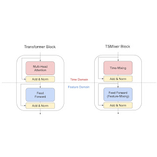
In our analysis, we show that under common assumptions of temporal patterns, linear models have naïve solutions to perfectly recover the time series or place bounds on the error, which means they are great solutions for learning static temporal patterns of univariate time series more effectively. In contrast, it is non-trivial to find similar solutions for attention mechanisms, as the weights applied to each time step are dynamic. Consequently, we develop a new architecture by replacing Transformer attention layers with linear layers. The resulting TSMixer model, which is similar to the computer vision MLP-Mixer method, alternates between applications of the multi-layer perceptron in different directions, which we call time-mixing and feature-mixing, respectively. The TSMixer architecture efficiently captures both temporal patterns and cross-variate information, as shown in the figure below. The residual designs ensure that TSMixer retains the capacity of temporal linear models while still being able to exploit cross-variate information.
 |
| Transformer block and TSMixer block architectures. TSMixer replaces the multi-head attention layer with time-mixing, a linear model applied on the time dimension. |
 |
| Comparison between data-dependent (attention mechanisms) and time-step-dependent (linear models). This is an example of forecasting the next time step by learning the weights of the previous three time steps. |
Evaluation on long-term forecasting benchmarks
We evaluate TSMixer using seven popular long-term forecasting datasets (ETTm1, ETTm2, ETTh1, ETTh2, Electricity, Traffic, and Weather), where recent research has shown that univariate linear models outperform advanced multivariate models with large margins. We compare TSMixer with state-of-the-art multivariate models (TFT, FEDformer, Autoformer, Informer), and univariate models, including linear models and PatchTST. The figure below shows the average improvement of mean squared error (MSE) by TSMixer compared with others. The average is calculated across datasets and multiple forecasting horizons. We demonstrate that TSMixer significantly outperforms other multivariate models and performs on par with state-of-the-art univariate models. These results show that multivariate models are capable of performing as well as univariate models.
 |
| The average MSE improvement of TSMixer compared with other baselines. The red bars show multivariate methods and the blue bars show univariate methods. TSMixer achieves significant improvement over other multivariate models and achieves comparable results to univariate models. |
Ablation study
We performed an ablation study to compare TSMixer with TMix-Only, a TSMixer variant that consists of time mixing layers only. The results show that TMix-Only performs almost the same as TSMixer, which means the additional feature mixing layers do not improve the performance and confirms that cross-variate information is less beneficial on popular benchmarks. The results validate the superior univariate model performance shown in previous research. However, existing long-term forecasting benchmarks are not well representative of the need for cross-variate information in some real-world applications where time series may be intermittent or sparse, hence temporal patterns may not be sufficient for forecasting. Therefore, it may be inappropriate to evaluate multivariate forecasting models solely on these benchmarks.
Evaluation on M5: Effectiveness of cross-variate information
To further demonstrate the benefit of multivariate models, we evaluate TSMixer on the challenging M5 benchmark, a large-scale retail dataset containing crucial cross-variate interactions. M5 contains the information of 30,490 products collected over 5 years. Each product description includes time series data, like daily sales, sell price, promotional event information, and static (non-time-series) features, such as store location and product category. The goal is to forecast the daily sales of each product for the next 28 days, evaluated using the weighted root mean square scaled error (WRMSSE) from the M5 competition. The complicated nature of retail makes it more challenging to forecast solely using univariate models that focus on temporal patterns, so multivariate models with cross-variate information and even auxiliary features are more essential.
First, we compare TSMixer to other methods only considering the historical data, such as daily sales and historical sell prices. The results show that multivariate models outperforms univariate models significantly, indicating the usefulness of cross-variate information. And among all compared methods, TSMixer effectively leverages the cross-variate information and achieves the best performance.
Additionally, to leverage more information, such as static features (e.g., store location, product category) and future time series (e.g., a promotional event scheduled in coming days) provided in M5, we propose a principle design to extend TSMixer. The extended TSMixer aligns different types of features into the same length, and then applies multiple mixing layers to the concatenated features to make predictions. The extended TSMixer architecture outperforms models popular in industrial applications, including DeepAR and TFT, showcasing its strong potential for real-world impact.
 |
| The architecture of the extended TSMixer. In the first stage (align stage), it aligns the different types of features into the same length before concatenating them. In the second stage (mixing stage) it applies multiple mixing layers conditioned with static features. |
 |
| The WRMSSE on M5. The first three methods (blue) are univariate models. The middle three methods (orange) are multivariate models that consider only historical features. The last three methods (red) are multivariate models that consider historical, future, and static features. |
Conclusion
We present TSMixer, an advanced multivariate model that leverages linear model characteristics and performs as well as state-of-the-art univariate models on long-term forecasting benchmarks. TSMixer creates new possibilities for the development of time series forecasting architectures by providing insights into the importance of cross-variate and auxiliary information in real-world scenarios. The empirical results highlight the need to consider more realistic benchmarks for multivariate forecasting models in future research. We hope that this work will inspire further exploration in the field of time series forecasting, and lead to the development of more powerful and effective models that can be applied to real-world applications.
Acknowledgements
This research was conducted by Si-An Chen, Chun-Liang Li, Nate Yoder, Sercan O. Arik, and Tomas Pfister.
 Ransomware attacks have become increasingly popular, more sophisticated, and harder to detect. For example, in 2022, a destructive ransomware attack took 233…
Ransomware attacks have become increasingly popular, more sophisticated, and harder to detect. For example, in 2022, a destructive ransomware attack took 233 days to identify and 91 days to contain, for a total lifecycle of 324 days. Going undetected for this amount of time can cause irreversible damage. Faster and smarter detection capabilities are critical to addressing these attacks.
Behavioral ransomware detection with NVIDIA DPUs and GPUs
Adversaries and malware are evolving faster than defenders, making it hard for security teams to track changes and maintain signatures for known threats. To address this, a combination of AI and advanced security monitoring is needed. Developers can build solutions for detecting ransomware attacks faster using advanced technologies including NVIDIA BlueField Data Processing Units (DPUs), the NVIDIA DOCA SDK with DOCA App Shield, and NVIDIA Morpheus cybersecurity AI framework.
Intrusion detection with BlueField DPU
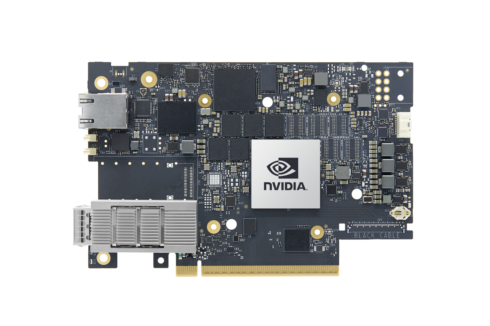
BlueField DPUs are ideal for enabling best-in-class, zero-trust security, and extending that security to include host-based protection. With built-in isolation, this creates a separate trust domain from the host system, where intrusion detection system (IDS) security agents are deployed. If a host is compromised, the isolation layer between the security control agents on the DPU and the host prevents the attack from spreading throughout the data center.
DOCA App-Shield is one of the libraries provided with the NVIDIA DOCA software framework. It is a security framework for host monitoring, enabling cybersecurity vendors to create IDS solutions that can quickly identify an attack on any physical server or virtual machine.
DOCA App-Shield runs on the NVIDIA DPU as an out-of-band (OOB) device in a separate domain from the host CPU and OS and is:
- Resilient against attacks on a host machine.
- Least disruptive to the execution of host applications.
DOCA App Shield exposes an API to users developing security applications. For detecting malicious activities from the DPU Arm processor, it uses DMA without involving the host OS or CPU. In contrast, a standard agent of anti-virus or endpoint-detection-response runs on the host and can be seen or compromised by an attacker or malware.
Morpheus AI framework for cybersecurity
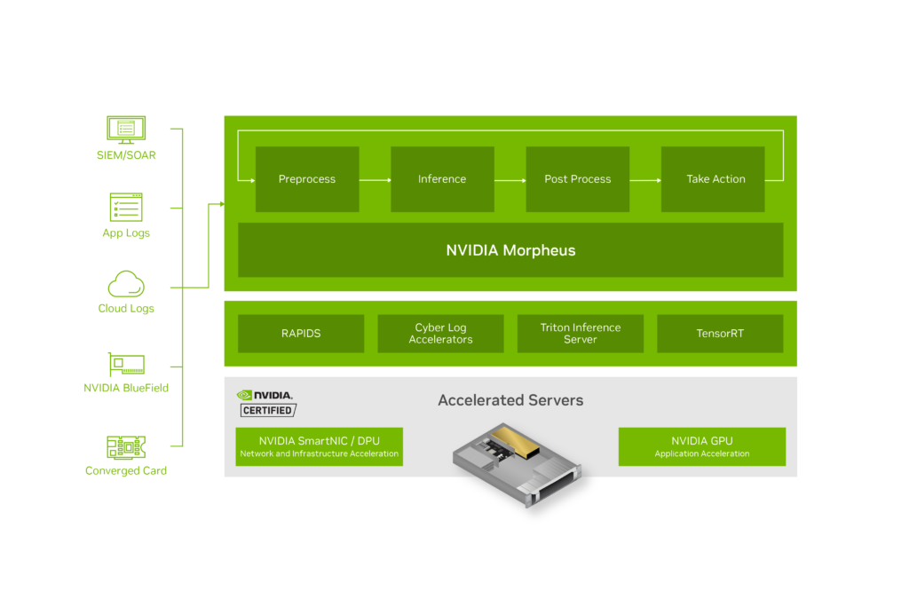
Morpheus is part of the NVIDIA AI Enterprise software product family and is designed to build complex ML and AI-based pipelines. It provides significant acceleration of AI pipelines to deal with high data volumes, classify data, and identify anomalies, vulnerabilities, phishing, compromised machines, and many other security issues.
Morpheus can be deployed on-premise with a GPU-accelerated server like the NVIDIA EGX Enterprise Platform, and it is also accessible through cloud deployment.
Addressing ransomware with AI
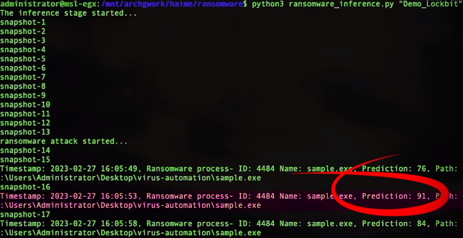
One of the pretrained AI models in Morpheus is the ransomware detection pipeline that leverages NVIDIA DOCA App-Shield as a data source. This brings a new level of security for detecting ransomware attacks that were previously impossible to detect in real time.
Inside BlueField DPU
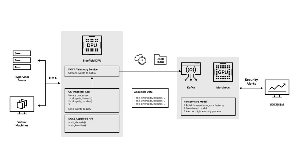
BlueField DPU offers the new OS-Inspector app to leverage DOCA App-Shield host monitoring capabilities and enables a constant collection of OS attributes from the monitored host or virtual machine. OS-Inspector app is now available through early access. Contact us for more information.
The collected operating system attributes include processes, threads, libraries, handles, and vads (for a complete API list, see the App-Shield programming guide).
OS-Inspector App then uses DOCA Telemetry Service to stream the attributes to the Morpheus inference server using the Kafka event streaming platform.
Inside the Morpheus Inference Framework
The Morpheus ransomware detection AI pipeline processes the data using GPU acceleration and feeds the data to the ransomware detection AI model.
This tree-based model detects ransomware attacks based on suspicious attributes in the servers. It uses N-gram features to capture the change in attributes through time and detect any suspicious anomaly.
When an attack is detected, Morpheus generates an inference event and triggers a real-time alert to the security team for further mitigation steps.
FinSec lab use case
NVIDIA partner FinSec Innovation Lab, a joint venture between Mastercard and Enel X, demonstrated their solution for combating ransomware attacks at NVIDIA GTC 2023.
FinSec ran a POC, which used BlueField DPUs and the Morpheus cybersecurity AI framework to train a model that detected a ransomware attack in less than 12 seconds. This real-time response enabled them to isolate a virtual machine and save 80% of the data on the infected servers.
Learn more
BlueField DPU running DOCA App Shield enables OOB host monitoring. Together with Morpheus, developers can quickly build AI models to protect against cyber attacks, better than ever before. OS-Inspector app is now available through early access. Contact us for more information.
 Extract-transform-load (ETL) operations with GPUs using the NVIDIA RAPIDS Accelerator for Apache Spark running on large-scale data can produce both cost savings…
Extract-transform-load (ETL) operations with GPUs using the NVIDIA RAPIDS Accelerator for Apache Spark running on large-scale data can produce both cost savings and performance gains. We demonstrated this in our previous post, GPUs for ETL? Run Faster, Less Costly Workloads with NVIDIA RAPIDS Accelerator for Apache Spark and Databricks. In this post, we dive deeper to identify precisely which Apache Spark SQL operations are accelerated for a given processing architecture.
This post is part of a series on GPUs and extract-transform-load (ETL) operations.
Migrating ETL to GPUs
Should all ETL be migrated to GPUs? Or is there an advantage to evaluating which processing architecture is best suited to specific Spark SQL operations?
CPUs are optimized for sequential processing with significantly fewer yet faster individual cores. There are clear computational advantages for memory management, handling I/O operations, running operating systems, and so on.
GPUs are optimized for parallel processing with significantly more yet slower cores. GPUs excel at rendering graphics, training, machine learning and deep learning models, performing matrix calculations, and other operations that benefit from parallelization.
Experimental design
We created three large, complex datasets modeled after real client retail sales data using computationally expensive ETL operations:
- Aggregation (SUM + GROUP BY)
- CROSS JOIN
- UNION
Each dataset was specifically curated to test the limits and value of specific Spark SQL operations. All three datasets were modeled based on a transactional sales dataset from a global retailer. The row size, column count, and type were selected to balance experimental processing costs while performing tests that would demonstrate and evaluate the benefits of both CPU and GPU architectures under specific operating conditions. See Table 1 for data profiles.
| Operation | Rows | # COLUMNS: Structured data | # COLUMNS: Unstructured data | Size (MB) |
| Aggregation (SUM + GROUP BY) | 94.4 million | 2 | 0 | 3,200 |
| CROSS JOIN | 63 billion | 6 | 1 | 983 |
| UNION | 447 million | 10 | 2 | 721 |
The following computational configurations were evaluated for this experiment:
- Worker and driver type
- Workers [minimum and maximum]
- RAPIDS or Photon deployment
- Maximal hourly limits on Databricks units (DBUs)—a proprietary measure of Databricks compute cost
| Worker and driver type | Workers [min/max] | RAPIDS Accelerator / PHOTON | Max DBUs / hour |
| Standard_NC4as_T4_v3 | 1/1 | RAPIDS Accelerator | 2 |
| Standard_NC4as_T4_v3 | 2/8 | RAPIDS Accelerator | 9 |
| Standard_NC8as_T4_v3 | 2/2 | RAPIDS Accelerator | 4.5 |
| Standard_NC8as_T4_v3 | 2/8 | RAPIDS Accelerator | 14 |
| Standard_NC16as_T4_v3 | 2/2 | RAPIDS Accelerator | 7.5 |
| Standard_NC16as_T4_v3 | 2/8 | RAPIDS Accelerator | 23 |
| Standard_E16_v3 | 2/2 | Photon | 24 |
| Standard_E16_v3 | 2/8 | Photon | 72 |
Other experimental considerations
In addition to building industry-representative test datasets, other experimental factors are listed below.
- Datasets are run using several different worker and driver configurations on pay-as-you-go instances–as opposed to spot instances–as their inherent availability establishes pricing consistency across experiments.
- For GPU testing, we leveraged RAPIDS Accelerator on T4 GPUs, which are optimized for analytics-heavy loads, and carry a substantially lower cost per DBU.
- The CPU worker type is an in-memory optimized architecture which uses Intel Xeon Platinum 8370C (Ice Lake) CPUs.
- We also leveraged Databricks Photon, a native CPU accelerator solution and accelerated version of their traditional Java runtime, rewritten in C++.
These parameters were chosen to ensure experimental repeatability and applicability to common use cases.
Results
To evaluate experimental results in a consistent fashion, we developed a composite metric named adjusted DBUs per minute (ADBUs). ADBUs are based on DBUs and computed as follows:

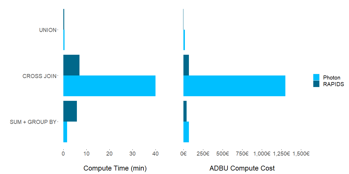
Experimental results demonstrate that there is no computational Spark SQL task in which one chipset–GPU or CPU–dominates. As Figure 1 shows, dataset characteristics and the suitability of a cluster configuration have the strongest impact on which framework to choose for a specific task. Although unsurprising, the question remains: which ETL processes should be migrated to GPUs?
UNION operations
Although RAPIDS Accelerator on T4 GPUs generate results having both lower costs and execution times with UNION operations, the difference when compared with CPUs is negligible. Moving an existing ETL pipeline from CPUs to GPUs seems unwarranted for this combination of dataset and Spark SQL operation. It is likely–albeit untested by this research–that a larger dataset may generate results that warrant a move to GPUs.
CROSS JOIN operations
For the compute-heavy CROSS JOIN operation, we observed an order of magnitude of both time and cost savings by employing RAPIDS Accelerator (GPUs) over Photon (CPUs).
One possible explanation for these performance gains is that the CROSS JOIN is a Cartesian product that involves an unstructured data column being multiplied with itself. This leads to exponentially increasing complexity. The performance gains of GPUs are well suited for this type of large-scale parallelizable operation.
The main driver of cost differences is that the CPU clusters we experimented with had a much higher DBU rating than the chosen GPU clusters.
SUM + GROUP BY operations
For aggregation operations (SUM + GROUP BY), we observed mixed results. Photon (CPUs) delivered notably faster compute times, whereas RAPIDS Accelerator (GPUs) provided lower overall costs. Looking at individual experimental runs, we observed that the higher Photon costs result in higher DBUs, whereas the costs associated with T4s are significantly lower.
This explains the lower overall cost using RAPIDS Accelerator in this part of the experiment. In summary, if speed is the objective, Photon is the clear winner. More price-conscious users may prefer the longer compute times of RAPIDS Accelerator for notable cost savings.
Deciding which architecture to use
The CPU cluster gained performance in execution time in the commonly used aggregation (SUM + GROUP BY) experiment. However, this came at the price of higher associated cluster costs. For CROSS JOINs, a less common high-compute and highly-parallelizable operation, GPUs dominated both in higher speed and lower costs. UNIONs showed negligible comparative differences in compute time and cost.
Where GPUs (and by association RAPIDS Accelerator) will excel depends largely on the data structure, the scale of the data, the ETL operation(s) performed, and the user’s technical depth.
GPUs for ETL
In general, GPUs are well suited to large, complex datasets and Spark SQL operations that are highly parallelizable. The experimental results suggest using GPUs for CROSS JOIN situations, as they are amenable to parallelization, and can also scale easily as data grows in size and complexity.
It is important to note the scale of data is less important than the complexity of the data and the selected operation, as shown in the SUM + GROUP BY experiment. (This experiment involved more data, but less computational complexity compared to CROSS JOINs.) You can work with NVIDIA free of charge to estimate expected GPU acceleration gains based on analyses of Spark log files.
CPUs for ETL
Based on the experiments, certain Spark SQL operations such as UNIONs showed a negligible difference in cost and compute time. A shift to GPUs may not be warranted in this case. Moreover, for aggregations (SUM + GROUP BY), a conscious choice of speed over cost can be made based on situational requirements, where CPUs will execute faster, but at a higher cost.
In cases where in-memory calculations are straightforward, staying with an established CPU ETL architecture may be ideal.
Discussion and future considerations
This experiment explored one-step Spark SQL operations. For example, a singular CROSS JOIN, or a singular UNION, omitting more complex ETL jobs that involve multiple steps. An interesting future experiment might include optimizing ETL processing at a granular level, sending individual SparkSQL operations to CPUs or GPUs in a single job or script, and optimizing for both time and compute cost.
A savvy Spark user might try to focus on implementing scripting strategies to make the most of the default runtime, rather than implementing a more efficient paradigm. Examples include:
- Spark SQL join strategies (broadcast join, shuffle merge, hash join, and so on)
- High-performing data structures (storing data in parquet files that are highly performant in a cloud architecture as compared to text files, for example)
- Strategic data caching for reuse
The results of our experiment indicate that leveraging GPUs for ETL can supply additional performance sufficient to warrant the effort to implement a GPU architecture.
Although supported, RAPIDS Accelerator for Apache Spark is not available by default on Azure Databricks. This requires the installation of .jar files that may necessitate some debugging. This tech debt was largely paid going forward, as subsequent uses of RAPIDS Accelerator were seamless and straightforward. NVIDIA support was always readily available to help if and when necessary.
Finally, we opted to keep all created clusters under 100 DBUs per hour to manage experimental costs. We tried only one size of Photon cluster. Experimental results may change by varying the cluster size, number of workers, and other experimental parameters. We feel these results are sufficiently robust and relevant for many typical use cases in organizations running ETL jobs.
Conclusion
NVIDIA T4 GPUs, designed specifically for analytics workloads, accomplish a leap in the price/performance ratio associated with leveraging GPU-based compute. NVIDIA RAPIDS Accelerator for Apache Spark, especially when run on NVIDIA T4 GPUs, has the potential to significantly reduce costs and execution times for certain common ETL SparkSQL operations, particularly those that are highly parallelizable.
To implement this solution on your own Apache Spark workload with no code changes, visit the NVIDIA/spark-rapids-examples GitHub repo or the Apache Spark tool page for sample code and applications that showcase the performance and benefits of using RAPIDS Accelerator in your data processing or machine learning pipelines.
Before she entered high school, Ge Dong wanted to be a physicist like her mom, a professor at Shanghai Jiao Tong University.
Rafi Nizam is an award-winning independent animator, director, character designer and more. He’s developed feature films at Sony Pictures, children’s series and comedies at BBC and global transmedia content at NBCUniversal.
 On Sept. 12, learn about the connection between MATLAB and NVIDIA Isaac Sim through ROS.
On Sept. 12, learn about the connection between MATLAB and NVIDIA Isaac Sim through ROS.
With coral reefs in rapid decline across the globe, researchers from the University of Hawaii at Mānoa have pioneered an AI-based surveying tool that monitors reef health from the sky. Using deep learning models and high-resolution satellite imagery powered by NVIDIA GPUs, the researchers have developed a new method for spotting and tracking coral reef Read article >
Creating 3D scans of physical products can be time consuming. Businesses often use traditional methods, like photogrammetry-based apps and scanners, but these can take hours or even days. They also don’t always provide the 3D quality and level of detail needed to make models look realistic in all its applications. Italy-based startup Covision Media is Read article >
Underscoring NVIDIA’s growing relationship with the global technology superpower, Indian Prime Minister Narendra Modi met with NVIDIA founder and CEO Jensen Huang Monday evening. The meeting at 7 Lok Kalyan Marg — as the Prime Minister’s official residence in New Delhi is known — comes as Modi prepares to host a gathering of leaders from Read article >