I am a beginner. I have installed Tensorflow version 2.6.0 and cuda version 11.7. However, tensorflow is not utilizing GPU. When I use tf.config.list_physical_devices(‘GPU’), it gives an empty object. Could anyone help me with this?
My question is linked to a question I asked recently: post
I need to loop over individual samples when training due to too large a batch size to hold in memory. I have had good success generating reproducible losses and and accumulated gradients with one of the training loops I am carrying out – and, applied gradients to weights are accurate (plus floating point errors) –
another custom loop I am carrying out on a batch is the mean squared error between a predicted label and the real label. Again, I need to iterate over the batch of samples manually due to a large batch size. To confirm it works, and I get the same losses and gradients, I am comparing my custom loop on a batch of 100 samples so i can compare both methods using ‘GradientTape()’
My code snippet is as follows: for batch training:
accum_gradient_val = [(acum_grad + grad) for acum_grad, grad in zip(accum_gradient_val, gradients)]
accum_gradient_vals_final = [this_grad / steps_per_epoch for this_grad in accum_gradient_val]policy_optimizer_ind.apply_gradients(zip(accum_gradient_vals_final, train_vars_val))
mean_loss = tf.reduce_mean(value_loss_tracking)
forgive the lack of indentation, but both loops work fine (in bold is the loss) – however, when I look at the loss in my custom loop relative to the mean squared error in the batch loop, the values are different starting sometimes from one decimal place – and they do not look like floating point errors to me. i.e. 0.43429542 and 0.4318762 – these seem really different to me to be floating point errors – in the other custom loop, i see floating points changing after about 5 decimal places… this is not the case here. sometime i will even see losses like 0.39 compared 0.40 – this seems not right to me. does anybody if this makes sense, or agree that this does not look right? I have tried np.mean and np.square also – I have looked at source code and cannot see exactly how Tensorflow does this under the hood!
The last line std::unique_ptr<tflite::Interpreter> interpreter; is throwing an error, suggesting that interpreter, and associated classes, are undefined. This is the error:
/usr/bin/ld: tensorflow-lite/libtensorflow-lite.a(interpreter.cc.o): in function `tflite::Interpreter::SetProfilerImpl(std::unique_ptr<tflite::Profiler, std::default_delete<tflite::Profiler> >)': interpreter.cc:(.text+0x2a66): undefined reference to `tflite::profiling::RootProfiler::RemoveChildProfilers()' /usr/bin/ld: interpreter.cc:(.text+0x2a75): undefined reference to `tflite::profiling::RootProfiler::AddProfiler(std::unique_ptr<tflite::Profiler, std::default_delete<tflite::Profiler> >&&)' /usr/bin/ld: interpreter.cc:(.text+0x2ab2): undefined reference to `vtable for tflite::profiling::RootProfiler' /usr/bin/ld: interpreter.cc:(.text+0x2b19): undefined reference to `vtable for tflite::profiling::RootProfiler' /usr/bin/ld: tensorflow-lite/libtensorflow-lite.a(interpreter.cc.o): in function `tflite::Interpreter::~Interpreter()': interpreter.cc:(.text+0x307e): undefined reference to `vtable for tflite::profiling::RootProfiler' /usr/bin/ld: tensorflow-lite/libtensorflow-lite.a(interpreter.cc.o): in function `tflite::profiling::RootProfiler::~RootProfiler()': interpreter.cc:(.text._ZN6tflite9profiling12RootProfilerD0Ev[_ZN6tflite9profiling12RootProfilerD5Ev]+0x7): undefined reference to `vtable for tflite::profiling::RootProfiler' /usr/bin/ld: tensorflow-lite/libtensorflow-lite.a(interpreter.cc.o): in function `tflite::profiling::RootProfiler::~RootProfiler()': interpreter.cc:(.text._ZN6tflite9profiling12RootProfilerD2Ev[_ZN6tflite9profiling12RootProfilerD5Ev]+0x7): undefined reference to `vtable for tflite::profiling::RootProfiler' collect2: error: ld returned 1 exit status make[2]: *** [CMakeFiles/model-verification.dir/build.make:247: model-verification] Error 1 make[1]: *** [CMakeFiles/Makefile2:1374: CMakeFiles/model-verification.dir/all] Error 2 make: *** [Makefile:149: all] Error 2
And I only get this error when I use `tflite::interpreter` despite having the correct `interpreter.h` file.
This is how I compile:
cmake ../tensorflow/lite/examples/model-verification/ make ./model-verification
This is my Cmake output:
cmake ../tensorflow/lite/examples/model-verification/ -- Setting build type to Release, for debug builds use'-DCMAKE_BUILD_TYPE=Debug'. CMake Warning at /home/me/tensorflow_src/build/abseil-cpp/CMakeLists.txt:74 (message): A future Abseil release will default ABSL_PROPAGATE_CXX_STD to ON for CMake 3.8 and up. We recommend enabling this option to ensure your project still builds correctly. -- Standard libraries to link to explicitly: none -- The Fortran compiler identification is GNU 11.2.0 -- Could NOT find CLANG_FORMAT: Found unsuitable version "0.0", but required is exact version "9" (found CLANG_FORMAT_EXECUTABLE-NOTFOUND) -- -- Configured Eigen 3.4.90 -- -- Proceeding with version: 2.0.6.v2.0.6 -- CMAKE_CXX_FLAGS: -std=c++0x -Wall -pedantic -Werror -Wextra -Werror=shadow -faligned-new -Werror=implicit-fallthrough=2 -Wunused-result -Werror=unused-result -Wunused-parameter -Werror=unused-parameter -fsigned-char -- Configuring done -- Generating done -- Build files have been written to: /home/onur/tensorflow_src/build
The CNN architecture defined using Keras’s functional API is:
input_ = Input(shape = (144, 144, 3), name = 'image') # name - An optional name string for the Input layer. Should be unique in # a model (do not reuse the same name twice). It will be autogenerated if it isn't provided. # Here 'image' is the Python3 dict's key used to map the data to one of the layer in the model. x = input_ # Define a conv block- x = Conv2D(filters = 64, kernel_size = 3, activation = 'relu')(x) x = BatchNormalization()(x) x = MaxPool2D(pool_size = 2)(x) x = Flatten()(x) # flatten the last pooling layer's output volume x = Dense(256, activation='relu')(x) # We are using a data generator which yields dictionaries. Using 'name' argument makes it # possible to map the correct data generator's output to the appropriate layer class_out = Dense(units = 9, activation = 'softmax', name = 'class_out')(x) # classification output box_out = Dense(units = 2, activation = 'linear', name = 'box_out')(x) # regression output # Define the CNN model- model = tf.keras.models.Model(input_, [class_out, box_out]) # since we have 2 outputs, we use a list
I am attempting to define it using Model sub-classing as:
class OD(Model): def __init__(self): super(OD, self).__init__() self.conv1 = Conv2D(filters = 64, kernel_size = 3, activation = None) self.bn = BatchNormalization() self.pool = MaxPool2D(pool_size = 2) self.flatten = Flatten() self.dense = Dense(256, activation = None) self.class_out = Dense(units = 9, activation = None, name = 'class_out') self.box_out = Dense(units = 2, activation = 'linear', name = 'box_out') def call(self, x): x = tf.nn.relu(self.bn(self.conv1(x))) x = self.pool(x) x = self.flatten(x) x = tf.nn.relu(self.dense(x)) x = [tf.nn.softmax(self.class_out(x)), self.box_out(x)] return x A batch of training data is obtained as: example, label = next(data_generator(batch_size = 32)) example.keys() # dict_keys(['image']) image = example['image'] image.shape # (32, 144, 144, 3) label.keys() # dict_keys(['class_out', 'box_out']) label['class_out'].shape, label['box_out'].shape # ((32, 9), (32, 2))
Is my Model sub-classing architecture equivalent to Keras’s functional API?
Experience the “Summer of Jetson” now through Sept. 30, with quizzes, prizes, and a project showcase to learn about the joys of working with Jetson Nano developer kit.
Object localization trained from scratch for emoji dataset in TensorFlow 2.8. Getting an IoU = 0.5969 and classification output accuracy = 100%. The code can be referred here. Though in fairness, I am using only 9 classes out of the emoji dataset. Thoughts?
In this post, we examine a method programmers can use to saturate memory bandwidth on a GPU.
Introduction
NVIDIA GPUs have enormous compute power and typically need to be fed data at high speed to deploy that power. That is possible, in principle, since GPUs also have high memory bandwidth, but sometimes they need the programmer’s help to saturate that bandwidth. In this blog post, we examine one method to accomplish that and apply it to an example taken from financial computing. We will explain under what circumstances this method can be expected to work well, and how to find out whether these circumstances apply to your workload.
Context
NVIDIA GPUs derive their power from massive parallelism. Many warps of 32 threads can be placed on a Streaming Multiprocessor (SM), awaiting their turn to execute. When one warp is stalled for whatever reason, the warp scheduler switches to another with zero overhead, making sure that the SM always has work to do. On the high-performance NVIDIA Ampere 100 (A100) GPU up to 64 active warps can share an SM, each with its own resources. On top of that, A100 has many SMs—108—that can all execute warp instructions simultaneously. Most instructions must operate on data, and that data almost always originates in the device memory (DRAM) attached to the GPU. One of the main reasons why even the abundance of warps on an SM can run out of work is because they are waiting on data to arrive from memory. If this happens and the bandwidth to memory is not fully utilized, it may be possible to reorganize the program to improve memory access and reduce warp stalls, which in turn makes the program complete faster.
First step: wide loads
In a previous blog post, we examined a workload that did not fully utilize the available compute and memory bandwidth resources of the GPU. We determined that prefetching data from memory before it is needed substantially reduced memory stalls and improved performance. When prefetching is not applicable, the quest is to determine what other factors may be limiting performance of the memory subsystem. One possibility is that the rate at which requests are made of that subsystem is too high. Intuitively, we may reduce the request rate by fetching multiple words per load instruction. It is best illustrated with an example.
In all code examples in this post, uppercase variables are compile-time constants. BLOCKDIMX assumes the value of the predefined variable blockDim.x. For some purposes, it must be a constant known at compile time, whereas for other purposes, it is useful for avoiding computations at run time. The original code looked like this, where index is a helper function to compute array indices. It implicitly assumes that just a single, one-dimensional thread block is being used, which is not the case for the motivating application from which it was derived. However, it reduces code clutter and does not change the argument.
for (pt = threadIdx.x; pt
Observe that each thread loads kmax consecutive values from the suggestively named small_array. This array is sufficiently small that it fits entirely in the L1 cache, but asking it to return data at a very high rate may become problematic. The following change recognizes that each thread can issue requests for two double-precision words in the same instruction if we restructure the code slightly and introduce the double2 data type, which is supported natively on NVIDIA GPUs; it stores two double-precision words in adjacent memory locations, which can be accessed with field selectors “x” and “y.” The reason this works is that each thread accesses successive elements of small_array. We call this technique wide loads. Notice that the inner loop over index “k” is now incremented by two instead of one.
for (pt = threadIdx.x; pt
A few caveats are in order. First, we did not check whether kmax is even. If not, the modified loop over k would execute an extra iteration, and we would need to write some special code to prevent that. Second, we did not confirm that small_array is properly aligned on a 16-byte boundary. If not, the wide loads would fail. If it was allocated using cudaMalloc, it would automatically be aligned on a 256-byte boundary. But if it was passed to the kernel using pointer arithmetic, some checks would need to be carried out.
Next, we inspect the helper function index and discover that it is linear in pt with coefficient 1. Consequently, we can apply a similar wide-load approach to values fetched from big_array by requesting two double-precision values in one instruction. The difference between accesses to big_array and to small_array is that now successive threads within a warp access adjacent array elements. The restructured code below doubles the increment of the loop over elements of array big_array, and now each thread processes two array elements in each iteration.
for (pt = 2*threadIdx.x; pt
The same caveats as before apply, and they should now be extended to parity of ptmax and alignment of big_array. Fortunately, the application from which this example was derived satisfies all the requirements. The figure below shows the duration (in nanoseconds) of a set of kernels that gets repeated identically multiple times in the application. The average speedup of the kernel was 1.63x for the combination of wide loads.
Figure 1. Reduction of kernel durations due to wide load
Second step: register use
We could be tempted to stop here and declare success, but a deeper analysis of the execution of the program, using NVIDIA Nsight Compute, shows that we have not fundamentally changed the rate of requests to the memory subsystem, even though we have halved the number of load instructions. The reason is that a warp load instruction—i.e. 32 threads simultaneously issuing load instructions—results in one or more sector requests, which is the actual unit of memory access processed by the hardware. Each sector is 32 bytes, so one warp load instruction of one 8-byte double-precision word per thread results in 8 sector requests (accesses are with unit stride), and one warp load instruction of double2 words results in 16 sector requests. The total number of sector requests is the same for plain and wide loads. So, what caused the performance improvement?
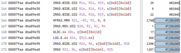
To understand the code behavior we need to consider a resource we have not yet discussed, namely registers. These are used to store the data loaded from memory and serve as input for arithmetic instructions. Registers are a finite resource. If a Streaming Multiprocessor (SM) hosts the maximum number of warps possible on the A100 GPU, 32 4-byte registers are available to each thread, which together can hold 16 double-precision words. The compiler that translates our code into machine language is aware of this and will limit the number of registers per thread. How do we determine the register use of our code and the role it plays in performance? We use the “source” view in Nsight Compute to see assembly code (“SASS”) and C source code side by side.
The innermost loop of the code is the one that is executed most, so if we select in the navigation menu “instructions executed” and subsequently ask to be taken to the line in the SASS code that has the highest number of those, we automatically land in the inner loop. If you are uncertain, you can compare SASS and the highlighted corresponding source code to confirm. Next, we identify in the SASS code of the inner loop all the instructions that load data from memory (LDG). Figure 2 shows a snippet of the SASS where we have panned around to find the start of the inner loop; it is on line 166 where the number of times an instruction is executed suddenly jumps to its maximum value.
LDG.E.64 is the instruction we are after. It LoaDs from Global memory (DRAM) a 64-bit word with an Extended address. The load of a wide word corresponds to LDG.E.128. The first parameter after the name of the load instruction (R34 in Figure 2) is the register that receives the value. Since a double-precision value occupies two adjacent registers, R35 is implied in the load instruction. Next, we compare for the three versions of our code (1. baseline, 2. wide loads of small_array, 3. wide loads of small_array and big_array) the way registers are used in the inner loop. Recall that the compiler tries to stay within limits and sometimes needs to play musical chairs with the registers. That is, if not enough registers are available to receive each unique value from memory it will reuse a register previously used in the inner loop.
The effect of that is that the previous value needs to be used by an arithmetic instruction so that it can be overwritten by the new value. At this time the load from memory needs to wait until that instruction completes: a memory latency is exposed. On all modern computer architectures, this latency constitutes a significant delay. On the GPU some of it can be hidden by switching to another warp, but often not all of it. Consequently, the number of times a register is reused in the inner loop can be an indication of the slowdown of the code.
With this insight, we analyze the three versions of our code and find that they experience 8, 6, and 3 memory latencies per inner loop, respectively, which explains the differences in performance shown in Figure 1. The main reason behind the different register reuse patterns is that when two plain loads are fused into a single wide load, typically fewer address calculations are needed, and the result of an address calculation also goes into a register. With more registers holding addresses, fewer addresses are left over to act as “landing zones” for values fetched from memory, and we lose seats in the musical chairs game; the register pressure grows.
Third step: launch bounds
We are not yet done. Now that we know the critical role registers play in the performance of our program, we review total register use by the three versions of the code. Easiest is to inspect Nsight Compute reports again. We find that the numbers of registers used are 40, 36, and 44, respectively.
The way the compiler determines these numbers is by using sophisticated heuristics that take a large number of factors into account, including how many active warps may be present on an SM, the number of unique values to be loaded in busy loops, and the number of registers required for each operation. If the compiler has no knowledge of the number of warps that may be present on an SM, it will try to limit the number of registers per thread to 32, because that is the number that would be available if the absolute maximum simultaneous number of warps allowed by the hardware (64) were present. In our case we did not tell the compiler what to expect, so it did its best, but evidently determined that the code generated using just 32 registers would be too inefficient.
However, the actual size of the thread block specified in the launch statement of the kernel is 1024 threads, so 32 warps. This means that if only a single thread block is present on the SM, each thread can use up to 64 threads. At 40, 36, and 44 registers per thread of actual use, not enough registers would be available to support two or more thread blocks per SM, so exactly one will be launched, and we leave 24, 28, and 20 registers per thread unused, respectively.
We can do a lot better by informing the compiler of our intent through the use of launch bounds. By telling the compiler the maximum number of threads in a thread block (1024) and also the minimum number of blocks to support simultaneously (1), it relaxes and is happy to use 63, 56, and 64 registers per thread, respectively.
Interestingly, the fastest version of the code is now the baseline version without any wide loads. While the combined wide loads without launch bounds gave a speedup of 1.64x, with launch bounds the speedup with wide loads becomes 1.76x, whereas the baseline code speeds up by 1.77x. This means we did not have to go to the trouble of modifying the kernel definition; merely supplying launch bounds was enough in this case to obtain optimal performance for this particular thread block size.
Experimenting a little more with thread block sizes and minimum number of threads blocks to be expected on the SM, we reach a speedup of 1.79x at 2 thread blocks of 512 threads each per SM, also for the baseline version without wide loads.
Conclusions
Efficient use of registers is critical to obtaining good performance of GPU kernels. Sometimes a technique called “wide loads” can give significant benefits. It reduces the number of memory addresses that are computed and need to be stored in registers, leaving a larger number of registers to receive data from memory. However, giving the compiler hints about the way you launch kernels in your application may give the same benefit without having to change the kernel itself.
Acknowledgements
The author would like to thank Mark Gebhart and Jerry Zheng of NVIDIA for providing the expertise to analyze register use in the example discussed in this blog.
This post introduces the adaptive routing technology for NVIDIA Spectrum Ethernet and provides preliminary performance benchmarks.
The NVIDIA accelerated AI platforms and offerings such as NVIDIA EGX, DGX, OVX, and NVIDIA AI for Enterprise require optimal performance out of data center networks. The NVIDIA Spectrum Ethernet platform delivers this performance through chip-level innovation.
Adaptive routing with RDMA over Converged Ethernet (RoCE) accelerates applications by reducing network congestion issues. This post introduces the adaptive routing technology for NVIDIA Spectrum Ethernet and provides some preliminary performance benchmarks.
What is slowing my network down?
You do not have to be a cloud service provider to benefit from scale-out networking. The networking industry has already figured out that traditional network architectures with Layer 2 forwarding and spanning trees are inefficient and struggle with scale. They transitioned to IP network fabrics.
This is a great start, but in some cases, it may not be enough to address the new type of applications and the amount of traffic introduced across data centers.
A key attribute of scalable IP networks is their ability to distribute massive amounts of traffic and flows across multiple hierarchies of switches.
In a perfect world, data flows are completely uncorrelated and are therefore well distributed, smoothly load balanced across multiple network links. This method relies on modern hash and multipath algorithms, including equal-cost multipath (ECMP). Operators benefit from high port count, fixed form-factor switches in data centers of any size.
However, there are many cases where this does not work, often including ubiquitous modern workloads like AI, cloud, and storage.
Figure 1. Introducing NVIDIA adaptive routing
The issue is the problem of limited entropy. Entropy is a way of measuring the richness and variety of flows traveling across a given network.
When you have thousands of flows that are randomly connected from clients around the globe, your network is said to have high entropy. However, when you have just a few large flows, which happens frequently with AI and storage workloads, the large flows dominate the bandwidth and therefore have low entropy. This low entropy traffic pattern is also known as an elephant flow distribution and is evident in many data center workloads.
So why does entropy matter?
Using legacy techniques with static ECMP, you need high entropy to spread traffic evenly across multiple links without congestion. However, in elephant flow scenarios, multiple flows can align to travel on the same link, creating an oversubscribed hot spot, or microburst. This results in congestion, increased latency, packet loss, and retransmission.
For many applications, performance is dictated not only by the average bandwidth of the network but also by the distribution of flow completion time. Longtails or outliers in the completion time distribution may decrease application performance significantly. Figure 2 shows the effect of low entropy on flow completion time.
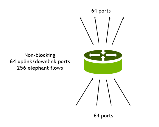
Figure 2. Example of network congestion
This example consists of a single top-of-rack switch with 128 ports of 100G.
64 ports are 100G downstream ports connecting to servers.
64 ports are 100G upstream ports connecting to Tier 1 switches.
Each downstream port receives traffic of four flows of equal bandwidth: 25G per flow for a total of 256 flows.
All traffic is handled through static hashing and ECMP.
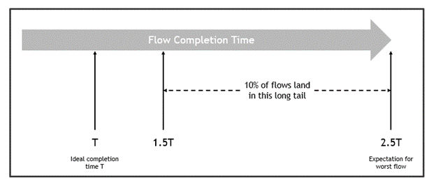
In the best case, the bandwidth available for this configuration is not oversubscribed so the following results are possible. In the worst-case scenario, flows can take up to 2.5x longer to complete compared to the ideal (Figure 3).
Figure 3. Flow completion times can vary significantly
In this case, a few ports are congested while others are unused. The last-flow (worst flow) expected duration is 250% of the expected first-flow duration. In addition, 10% of flows suffer from an expected flow completion time of more than 150%. That is, there is a long tail of flows where the completion time is longer than expected. To avoid congestion with high confidence (98%), you must reduce the bandwidth of all flows to under 50%.
Why are there many flows that suffer from high completion time? This is because some ports on the ECMP are highly congested. As flows finish transmission and release some port bandwidth, the lagging flows pass through the same congested ports, causing more congestion. This is because routing is static after the header has been hashed.
Adaptive routing
NVIDIA is introducing adaptive routing to Spectrum switches. With adaptive routing, traffic forwarding to an ECMP group selects the least-congested port for transmission. Congestion is evaluated based on egress queue loads, ensuring that an ECMP group is well-balanced regardless of the entropy level. An application that issues multiple requests to several servers receives the data with minimal time variation.
How is this achieved? For every packet forwarded to an ECMP group, the switch selects the port with the minimal load over its egress queue. The queues that are evaluated are those that match the packet quality of service.
By contrast, traditional ECMP makes the port decision based on the hashing method, which often fails to yield a clear comparison. As different packets of the same flow travel through different paths of the network, they may arrive out of order to their destination. At the RoCE transport layer, the NVIDIA ConnectX NIC takes care of the out-of-order packets and forwards the data to the application in order. This renders the magic of adaptive routing invisible to the application benefiting from it.
On the sender side, ConnectX can dynamically mark traffic for eligibility to network re-ordering, thus ensuring that inter-message ordering can be enforced when required. The switch adaptive routing classifier can classify only these marked RoCE traffic to be subjected to its unique forwarding.
Spectrum adaptive routing technology supports various network topologies. For typical topologies such as Clos (or leaf/spine), the distance of the various paths to a given destination is the same. Therefore, the switch transmits the packets through the least congested port. In other topologies where distances vary between paths, The switch prefers to send the traffic over the shortest path. If congestion occurs on the shortest path, then the least-congested alternative paths are selected. This ensures that the network bandwidth is efficiently used.
Workload results
NEEDS LEAD-IN SENTENCE
Storage
To verify the effect of adaptive routing in RoCE, we started by testing simple RDMA write test applications. In these tests, which ran on multiple 50 Gb/s hosts, we divided the hosts into pairs, and each pair sent each other large RDMA write flows for a long period of time. This type of traffic pattern is typical in storage application workloads.
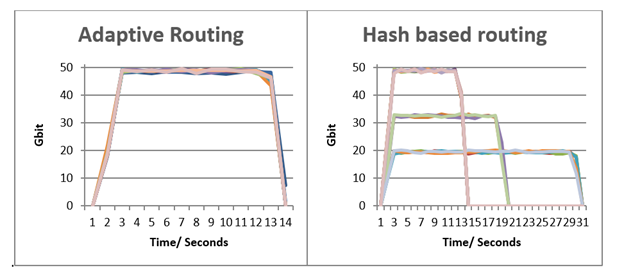
Figure 4 shows that the static, hash-based routing suffered from collisions on the uplink ports, causing increased flow completion time, reduced bandwidth, and reduced fairness between the flows. All problems were solved after moving to adaptive routing.
Figure 4. Adaptive routing for storage workloads
In the first graph, all flows completed at approximately the same time, with comparable peak bandwidth.
In the second graph, some of the flows achieved the same bandwidth and completion time, with other flows colliding, resulting in longer completion times and lower bandwidth. Indeed, in the ECMP case, some flows completed in an ideal completion time T of 13 seconds, while the worst-performing flows took 31 seconds, approximately 2.5x of T.
AI/HPC
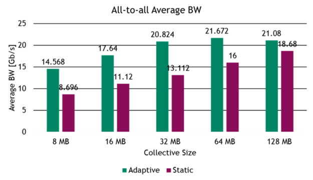
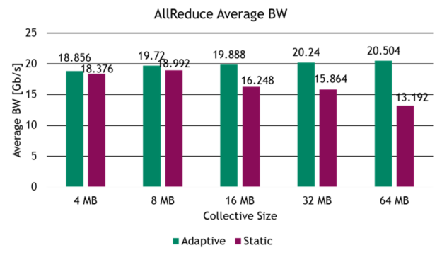
To continue with evaluating adaptive routing in RoCE workloads, we tested the performance gains for common AI benchmarks on a 32-server testbed, built with four NVIDIA Spectrum switches in a two-level, fat-tree network topology. The benchmark evaluates common collective operations and network traffic patterns found in distributed AI training and HPC workloads, such as all-to-all traffic and all-reduce collective operations.
Figure 5. Adaptive routing for AI: all-to-all
Figure 6. Adaptive routing for AI: all-reduce
Summary
In many cases, forwarding based on static hashes leads to high congestion and variable flow completion time. This reduces application-level performance.
NVIDIA Spectrum adaptive routing solves this issue. This technology increases the network’s used bandwidth, minimizes the variability of the flow completion time and, as a result, boosts the application performance.
Combining this technology with RoCE Out Of Order support from NVIDIA ConnectX NICs, the application is transparent to the technology used. This ensures that the NVIDIA Spectrum Ethernet platform delivers the accelerated Ethernet needed for maximum data center performance.
Overcome data challenges and build high-quality synthetic data to accelerate the training and accuracy of AI perception networks with Omniverse Replicator, available in beta.
Companies providing synthetic data generation tools and services, as well as developers, can now build custom physically accurate synthetic data generation pipelines with the Omniverse Replicator SDK. Built on the NVIDIA Omniverse platform, the Omniverse Replicator SDK is available in beta within Omniverse Code.
Omniverse Replicator is a highly extensible SDK built on a scalable Omniverse platform for physically accurate 3D synthetic data generation to accelerate training and performance of AI perception networks. Developers, researchers, and engineers can now use Omniverse Replicator to bootstrap and improve performance of existing deep learning perception models with large-scale photorealistic synthetic data.
Figure 1. Replicator uses the Omniverse open standards-based platform along with extensibility and scalability provided by OmniGraph and Farm architecture
Omniverse Replicator provides an extraordinary platform for developers to build synthetic data generation applications specific to their neural network’s requirements. Built on open standards like Universal Scene Description (USD), PhysX, and Material Definition Language (MDL), with easy to use python APIs, it’s also made for expandability, supporting custom randomizers, annotators, and writers. Supporting lightning fast data generation with a CUDA-based OmniGraph implementation of core annotator features means that output can be instantly previewed. When combined with Omniverse Farm and SwiftStack output, Replicator provides massive scalability in the cloud.
The Omniverse Replicator SDK is composed of six primary components for custom synthetic data workflows:
Semantic Schema Editor: With Semantic labeling of 3D assets and its prims, Replicator can annotate objects of interest during the rendering and data generation process. The Semantic Schema Editor provides a way to apply these labels to prims on the stage through a user interface.
Visualizer: This provides visualization capabilities for the semantic labels assigned to 3D assets along with annotations like 2D/3D bounding boxes, normals, depth, and more.
Randomizers: Domain randomization is one of the most important capabilities of Replicator. Using randomizers you can create randomized scenes, sampling from assets, materials, lighting, and camera positions among other randomization capabilities.
Omni.syntheticdata: This provides low-level integration with Omniverse RTX Renderer and OmniGraph computation graph system. It also powers Replicator’s ground truth extraction Annotators, passing Arbitrary Output Variables (AOVs) from the renderer through to the Annotators.
Annotators: These ingest AOVs and other output from the Omni.syntheticdata extension to produce precisely labeled annotations for deep neural network (DNN) training.
Writers: Process images and other annotations from the annotators, and produce DNN-specific data formats for training.
Synthetic data in AI training
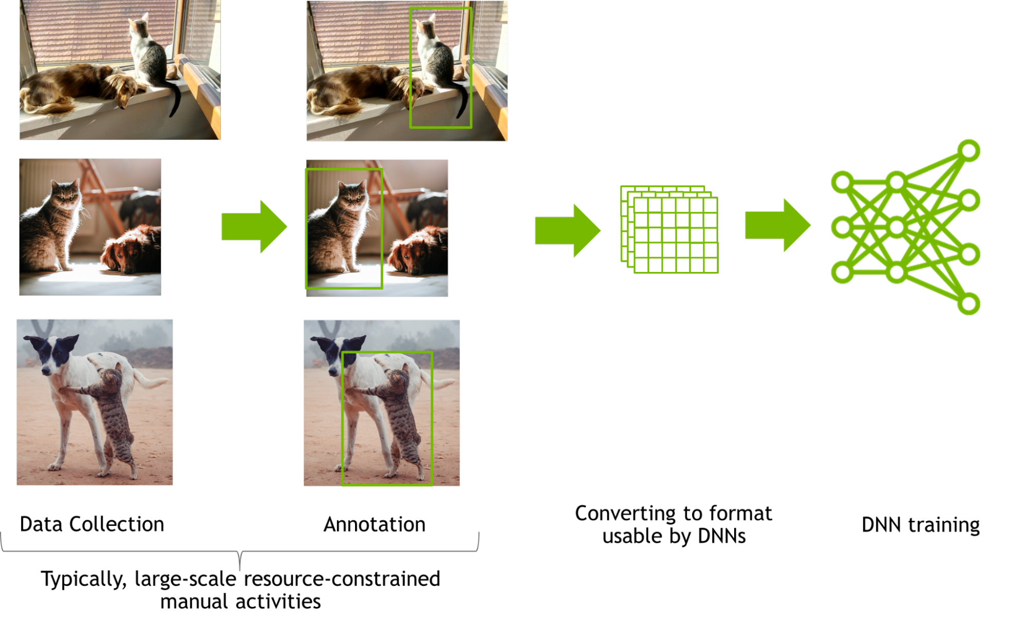
Training a DNN for perception tasks often involves manual collection of data from millions of images followed by manually annotating these images and optional augmentations.
Figure 2. Data collection and annotation tasks graph
Manual data collection and annotations are laborious and subjective. Collecting and annotating real images with even simple annotations like 2D bounding boxes at a large scale pose many logistical challenges. Involved annotations such as segmentation are resource constrained and are far less accurate when performed manually.
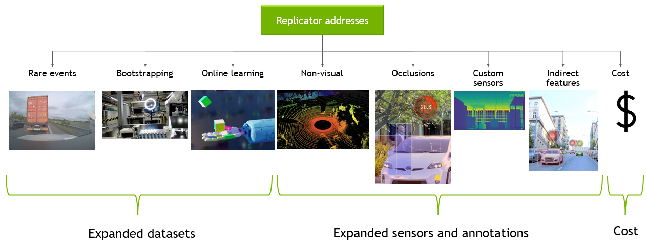
Figure 3. Complexities of Semantics Segmentation tasks
Once collected and annotated, the data is converted into the format usable by the DNN, and the DNN is then trained for the perception tasks. Hyperparameter tuning or changes in network architecture are typical next steps to optimize network performance. Analysis of the model performance may lead to potential changes in the dataset, but in most cases, this requires another cycle of manual data collection and annotation. This iterative cycle of manual data collection and annotation is expensive, tedious, and slow.
With synthetically generated data, teams can bootstrap and enhance large-scale training data generation with accurate annotations in a cost-effective manner. Plus, synthetic data generation also helps solve challenges related to long tail anomalies, lack of available training data, and online reinforcement learning. Unlike manually collected and annotated data, synthetically generated data has lower amortization cost, which is beneficial for typical iterative nature of the data collection/annotations and model training cycle.
Figure 4. Omniverse Replicator for large-scale training data generation with accurate annotations
Omniverse Replicator addresses these challenges by leveraging many of the core functionalities of the Omniverse platform and best practices including but not limited to physically accurate, photoreal datasets and access to very large datasets.
Physically accurate, photoreal datasets require accurate ray tracing and path tracing with RTX technologies, physically based materials, and physics engine—all core technologies of the Omniverse platform.
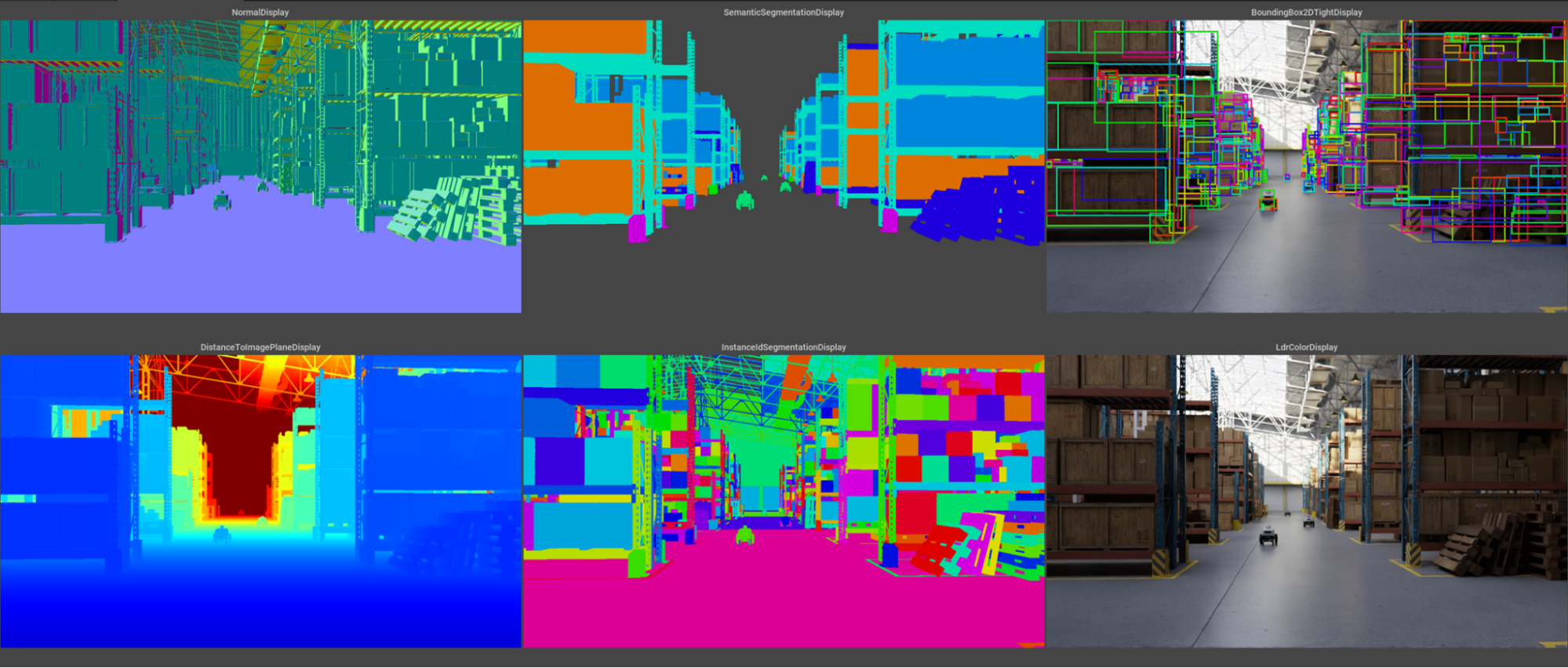
Figure 5. Enhanced sensor annotations in a warehouse scene using Omniverse Replicator
Based on Universal Scene Description (USD), Omniverse seamlessly connects to other 3D applications so developers can bring in custom-made content, or write their own tools to generate diverse domain scenes. Generating these assets is often a bottleneck, as it requires scaling across multiple GPUs and nodes.
Omniverse Replicator leverages Omniverse Farm, which lets teams use multiple workstations or servers together to power jobs like rendering or synthetic data generation. A synthetic data generation workflow is not “one and done.” To train a network with synthetic data successfully, the network has to be tested iteratively on a real dataset. Replicator provides this kind of data-centric AI training by converting simulated worlds into a set of learnable parameters.
Accelerate existing workflows with Omniverse Replicator and TAO Toolkit
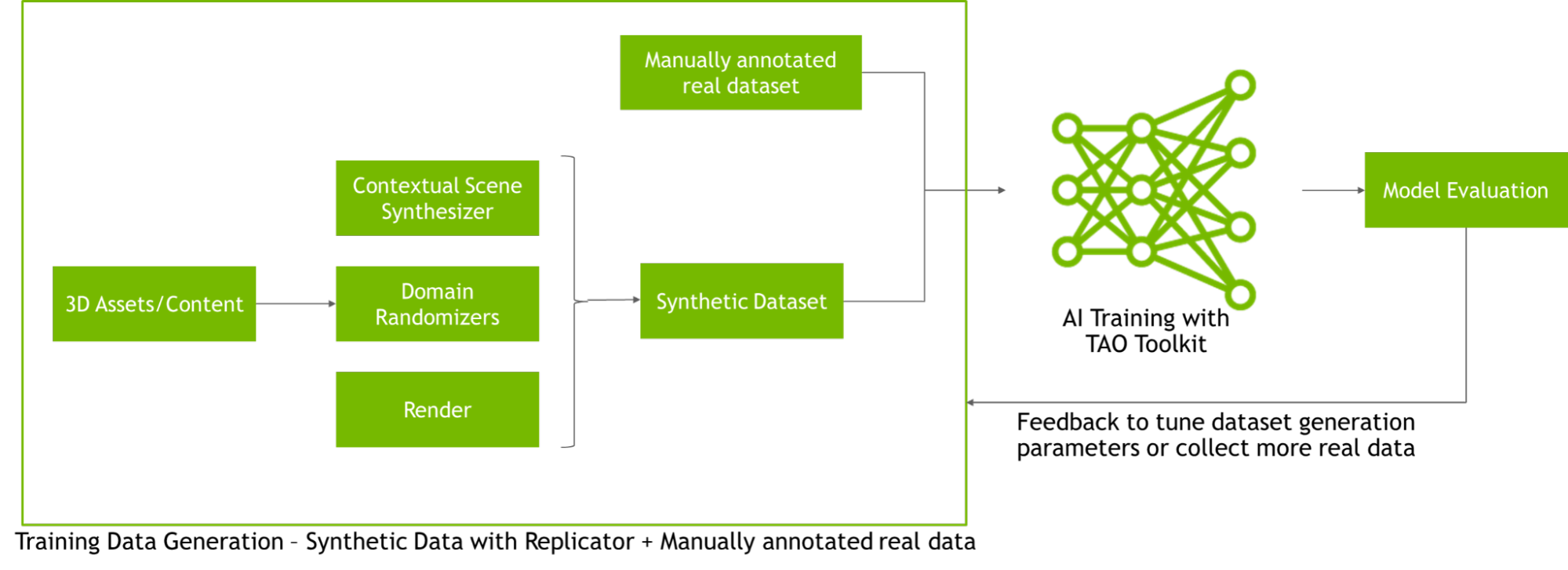
Developers, engineers, and researchers can integrate Omniverse Replicator with existing tools to speed up AI model training. For example, once synthetic data is generated, developers can train their AI models quickly using the NVIDIA TAO Toolkit. The TAO Toolkit leverages the power of transfer learning, for developers to train, adapt, and optimize models for their use-case, without prior AI expertise.
Figure 6. Omniverse Replicator and TAO toolkit workflow for synthetic data generation and model training
Building applications with Omniverse Replicator
Kinetic Vision is a systems integrator for large industrial customers in retail, intralogistics, consumer manufacturing, and consumer packaged goods. They are developing a new enterprise application based on the Omniverse Replicator SDK to provide high-quality synthetic data for customers as a service.
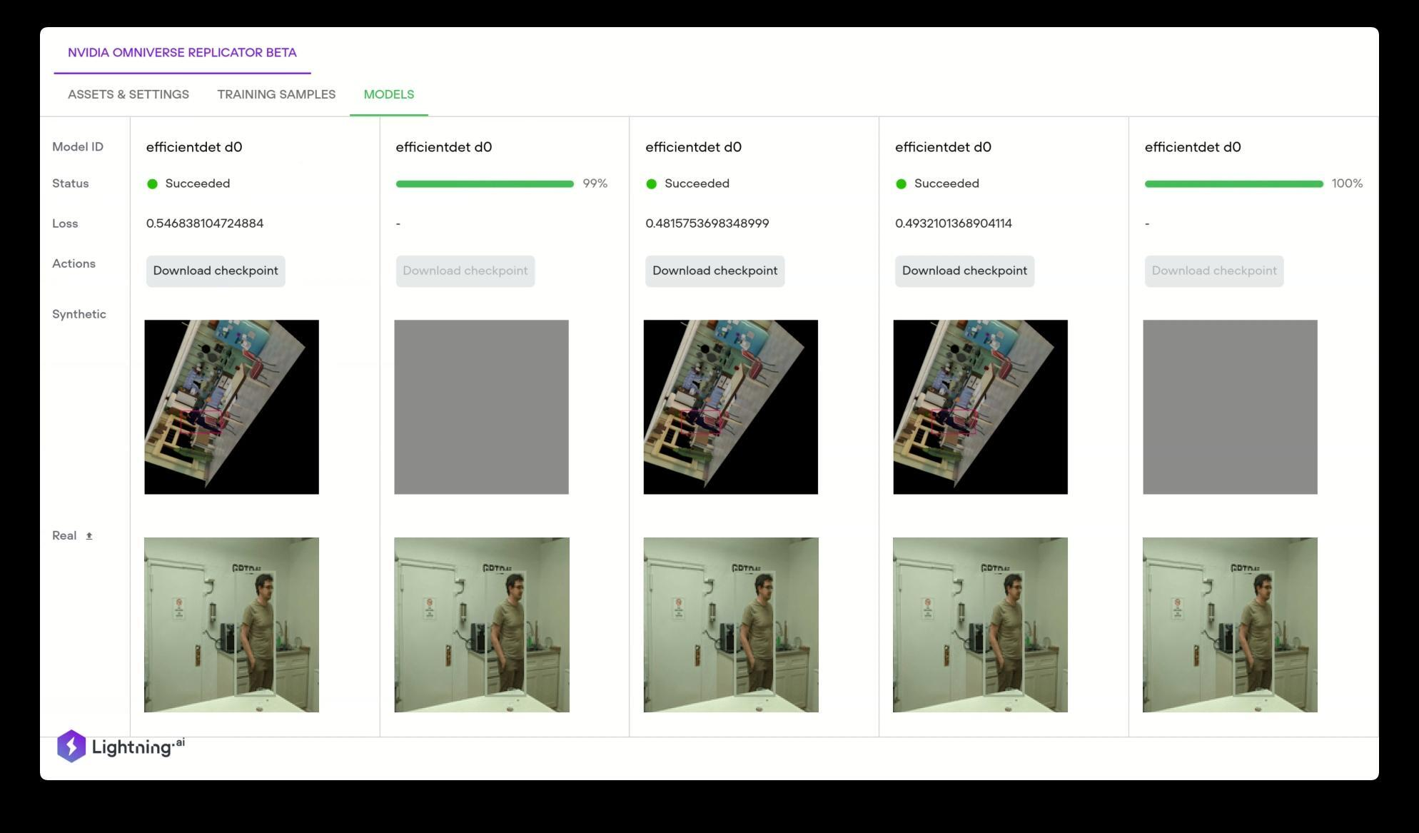
When data required to train deep learning models is unavailable, Omniverse Replicator generates synthetic data, which can be used to augment limited datasets. Lightning AI (formerly Grid.AI) uses the NVIDIA Omniverse Replicator to generate physically accurate 3D datasets based on Universal Scene Description (USD) that can be used to train these models. A user can simply drag and drop your 3D assets and after the dataset is generated a user can choose from the latest state-of-the-art computer vision models to train automatically on the synthetic data.
Figure 7. Lightning AI Application showing DNNs trained and tested on synthetic data generated by Replicator
At NVIDIA, the Isaac Sim and DRIVE Sim teams leveraged the Omniverse Replicator SDK to build domain-specific synthetic generation tools, the Isaac Replicator for robotics, and DRIVE Replicator for autonomous vehicle training. The Omniverse Replicator SDK provides a core set of functionalities for developers to build any domain specific synthetic data generation pipeline using all the benefits offered by the Omniverse platform. With Omniverse as a development platform for 3D simulation, rendering, and AI development capabilities, Replicator provides a custom synthetic data generation pipeline.
Figure 8. NVIDIA Isaac Sim (left) and DRIVE Sim (right) synthetic data capabilities built using Omniverse Replicator
Learn more by diving into the Omniverse Resource Center, which details how developers can build custom applications and extensions for the platform.
Follow Omniverse on Instagram, Twitter, YouTube, and Medium for additional resources and inspiration. Check out the Omniverse forums for expert guidance.

 Experience the “Summer of Jetson” now through Sept. 30, with quizzes, prizes, and a project showcase to learn about the joys of working with Jetson Nano developer kit.
 In this post, we examine a method programmers can use to saturate memory bandwidth on a GPU.
 This post introduces the adaptive routing technology for NVIDIA Spectrum Ethernet and provides preliminary performance benchmarks.
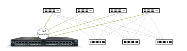

![How to Generate Images From Text Prompts with VQGAN-Clip, Python, and TensorFlow [Tutorial]](https://a.thumbs.redditmedia.com/n7t7yStrwe4vVyxBM1tFYeGkAr1Otm_qgzmpVuBnVa4.jpg "How to Generate Images From Text Prompts with VQGAN-Clip, Python, and TensorFlow [Tutorial]")
 Overcome data challenges and build high-quality synthetic data to accelerate the training and accuracy of AI perception networks with Omniverse Replicator, available in beta.
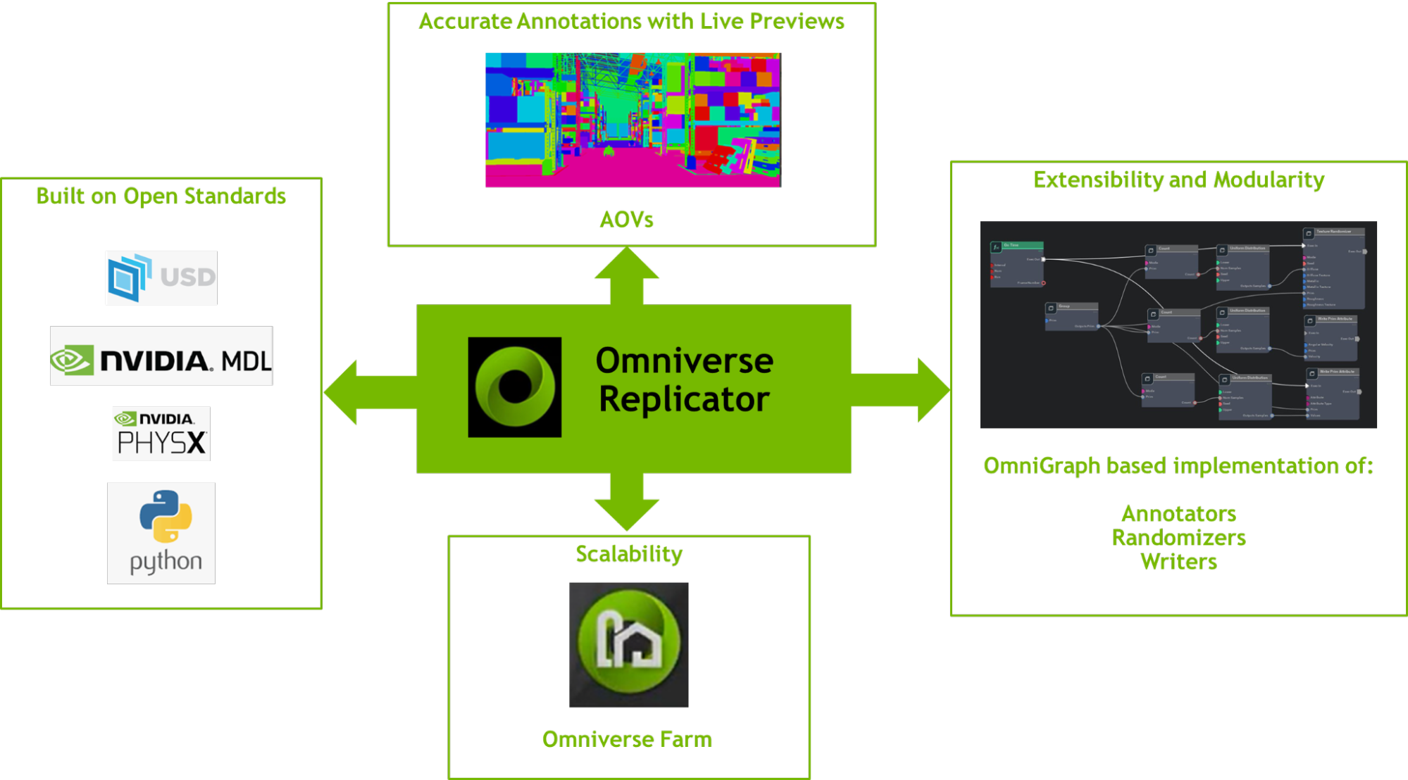

