I was learning about object detection for multiple classes. If given a cat image,it should detect a cat. If given a dog image, it should detect a dog. Here is a gist of what I did.
1) Created a dateset of dogs and labelled them. 2) Created a datset of cats and labelled them. 3) Put them both in a single folder ( dogs+cats) 4) Spllit them into train and test( 80,20) 4) Generated TF records. (test, train) 5) Downloaded pretrained ssd_mobilenetv2 from zoo, changed pipeline.config ( classes=2, batch_size=16, steps=2000) 6) Trained the model, ended at a total loss of 1.2 7) Exported the model to a .pb file 8) Tested the model by giving an image.
This is where, I am confused. If I give an image of a dog, the bounding box is showing that it is a cat, if I give an image of a cat it is shown that it is a dog. I am really confused as to where I made the mistake.
Did I make a mistake in the dataset preparation by creating the datesets separately and then merging them together? Or can anything else cause this.
A new approach to autonomous driving is pursuing a solo career. Researchers at MIT are developing a single deep neural network (DNN) to power autonomous vehicles, rather than a system of multiple networks. The research, published at COMPUTEX this week, used NVIDIA DRIVE AGX Pegasus to run the network in the vehicle, processing mountains of Read article >
NVIDIA SimNet is a physics-informed neural network (PINNs) toolkit, which addresses these challenges using AI and physics.
Today, NVIDIA announces the release of SimNet v21.06 for general availability, enabling physics simulations across a variety of use cases.
NVIDIA SimNet is a Physics-Informed Neural Networks (PINNs) toolkit for engineers, scientists, students, and researchers who either want to get started with AI-driven physics simulations, or would like to leverage a powerful framework to implement their domain knowledge to solve complex nonlinear physics problems with real-world applications.
V21.06 builds on a successful early access program of baseline features, and layers on additional new capabilities. This GA release introduces support for new physics such as Electromagnetics and 2D wave propagation, as well as delivers a new algorithm that enables wider number of use cases for simulating more complex Fluid-Thermal systems. New time stepping schemes have been implemented for solving temporal problems, treating time as both discrete and continuous.
Other features and enhancements include a gradient aggregation method for increased batch size on each GPU, adaptive sampling for increased point cloud density in regions of high losses, homoscedastic task uncertainty quantification for loss weighting, transfer learning algorithm enables rapid training for efficient surrogate-based parameterization of STL as well as constructive solid geometries and Polynomial Chaos Expansion method for assessing how uncertainties in a model input manifest in its output. SimNet v21.06 also expands the existing network architectures with Multiplicative Filter Networks.
SimNet v21.06 Highlights
Electromagnetics Frequency domain electromagnetic simulation can be carried out using SimNet v21.06. Solution of real form of frequency domain Maxwell’s equation is available either in scalar form (Helmholtz equation) for 1D, 2D and 3D cases, or in vector form for 3D case. The boundary conditions can be perfect electronic conductor (PEC) for 2D and 3D cases, radiation boundary (absorbing boundary) condition for 3D and waveguide port solver for 2D waveguide source. The implementation can solve for 2D TEz and TMz mode frequency domain electromagnetics and 3D electromagnetics in real form.
Time Stepping Scheme for Temporal Physics Transient simulations are required for many computational problems in such fields as fluid dynamics and electromagnetism. Until recently, neural network solvers have struggled to obtain accurate results. Using several innovations in this field, SimNet is now able solve a variety of transient problems to significantly greater degree of speed and accuracy. Shown below is Taylor-Green vortex decay using transient and turbulent Navier-Stokes simulation.
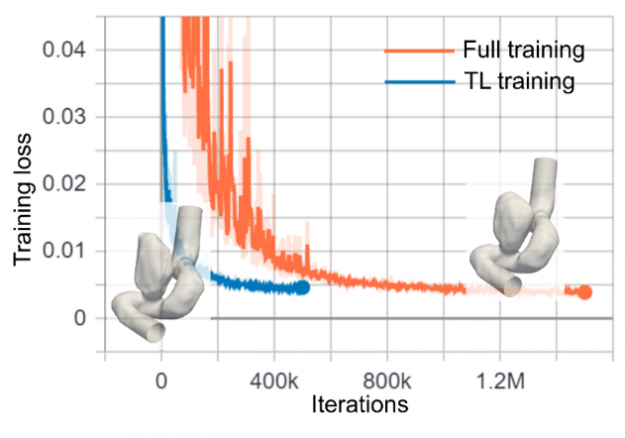
Transfer Learning In repetitive trainings, such as training for surrogate-based design optimization or uncertainty quantification, transfer learning reduces the time to convergence for neural network solvers. Once a model is trained for a single geometry, the trained model parameters are transferred to solve a different geometry, without having to train on the new geometry from scratch.
Transfer learning accelerates patient-specific intracranial aneurysm simulations.
Aneurysms with two different shapes.
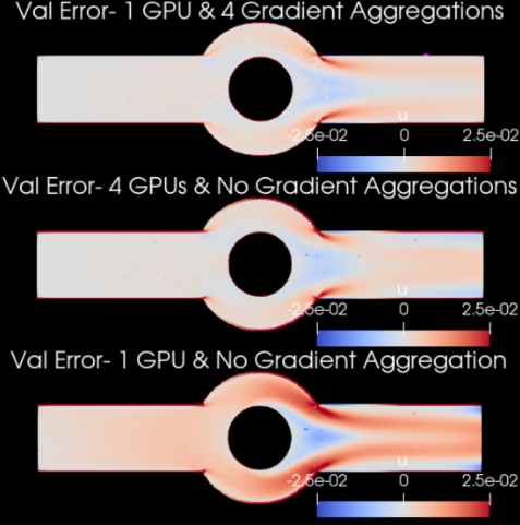
Gradient Aggregation Training of a neural network solver for complex problems requires a large batch size that can be beyond the available GPU memory limits. Increasing the number of GPUs can effectively increase the batch size but in case of limited GPU availability, you can use gradient aggregation. With gradient aggregation, the required gradients are computed in several forward/backward iterations using different mini batches of the point cloud and are then aggregated and applied to update the model parameters. This will, in effect, increase the batch size (although at the cost of increasing the training time).
Increasing the batch size can improve the accuracy of neural network solvers.
4 Gradient Aggregations on 1 GPU = 4 GPUs without Gradient Aggregations. These results are more accurate than the 1 GPU result without any Gradient Aggregation.
Recent SimNet On-Demand Technical Sessions
“Physics-Informed Neural Networks for Mechanics of Heterogenous Media” – IIT-Bombay presented a session on Physics-Informed Neural Networks for Mechanics of Heterogeneous Media. The PINN-based NVIDIA SimNet toolkit is used to develop a framework for the simulation of damage in elastic and elastoplastic materials. For verification, SimNet results are found in good agreement with the analytical solution based on Haghighat et al, 2020.
“Using Physics-Informed Neural Networks and SimNet to Accelerate Product Development” – Kinetic Vision presented a session on using Physics Informed Neural Networks and SimNet to accelerate product development where the Coanda effect, encountered in aerospace and several industrial applications, is simulated using SimNet. Both 2D and 3D geometries are constructed using SimNet’s internal Geometry module and simulated using modified Fourier Network Architecture. The results showed that qualitatively, the velocity flow field predicted by the commercial CFD code, Ansys Fluent and the trained SimNet PINN are very similar. Furthermore, Kinetic Vision did parametric simulations with SimNet and went a step further by taking these results and integrating them into CAD with SolidWorks for automated inference as well as providing a way for users to interact with SimNet from within Solidworks UI.
“Hybrid Physics-Informed Neural Networks for Digital Twin in Prognosis and Health Management” – University of Central Florida presented a session on Hybrid Physics-Informed Neural Networks for Digital Twin in Prognosis and Health Management where a Digital twin model is built to predict damage and fatigue crack growth in aircraft window panels. SimNet models are based in physics and this ensures accuracy needed for prognosis and health management of structural materials. Once SimNet models are trained, they can be used to perform fast and accurate computations as a function of different input conditions. SimNet also achieves good accuracy that the commercial solvers achieve with high degree of mesh refinement. With SimNet, they can scale the predictive model to a fleet of 500 aircraft and get predictions in less than 10 seconds as opposed to taking a few days to weeks if they were to perform the same computations using high-fidelity finite element models.
“Physics-Informed Neural Network for Flow and Transport in Porous Media” – Stanford University presented a session on Physics-Informed Deep Learning for Flow and Transport in Porous Media where a methodology is used to simulate a 2-phase immiscible transport problem (Buckley-Leverett). The model can produce an accurate physical solution both in terms of shock and rarefaction and honors the governing partial differential equation along with initial and boundary conditions. Read more about this on our NVIDIA blog here.
“AI-Accelerated Computational Science and Engineering Using Physics-Based Neural Networks” – NVIDIA presented a session on AI-Accelerated Computational Science and Engineering Using Physics-Based Neural Networks that covers state-of-the-art AI for addressing diverse areas of applications ranging from real-time simulation (e.g., digital twin and autonomous machines) to design space exploration (generative design and product design optimization), inverse problems (e.g., medical imaging, full wave inversion in oil and gas exploration) and improved science (e.g., micromechanics, turbulence) that are difficult to solve because of various gradients and discontinuities, due to physics laws and complex shapes.
To achieve state-of-the-art machine learning (ML) solutions, data scientists often build complex ML models. However, these techniques are computationally expensive, and until recently required extensive background knowledge, experience, and human effort. Recently, at GTC21, AWS Senior Data Scientist Nick Erickson gave a session sharing how the combination of AutoGluon, RAPIDS, and NVIDIA GPU computing simplifies … Continued
To achieve state-of-the-art machine learning (ML) solutions, data scientists often build complex ML models. However, these techniques are computationally expensive, and until recently required extensive background knowledge, experience, and human effort.
Recently, at GTC21, AWS Senior Data Scientist Nick Erickson gave a session sharing how the combination of AutoGluon, RAPIDS, and NVIDIA GPU computing simplifies achieving state-of-the-art ML accuracy, while improving performance and lowering costs. This post gives an overview of some key points from Nick’s session:
What is AutoML and what is different about AutoGluon?
How does AutoGluon outperform 99% of human data science teams in Kaggle prediction competitions with just three lines of code, without the need for expert knowledge?
How does the integration of AutoGluon with RAPIDS enable up to 40x faster training and 10x faster inference?
What is AutoGluon?
AutoGluon is an open-source AutoML library that enables easy-to-use and easy-to-extend AutoML with a focus on automated stack ensembling, deep learning, and real-world applications spanning text, image, and tabular data. Intended for both ML beginners and experts, AutoGluon enables you to:
Quickly prototype deep learning and classical ML solutions for your raw data with a few lines of code.
Automatically utilize state-of-the-art techniques (where appropriate) without expert knowledge.
Leverage automatic hyperparameter tuning, model selection/ensembling, architecture search, and data processing.
Easily improve/tune your bespoke models and data pipelines, or customize AutoGluon for your use case.
This post focuses on AutoGluon-Tabular, an AutoGluon API that requires only a few lines of Python to train highly accurate machine learning models on an unprocessed tabular dataset such as a CSV file. In order to understand how AutoGluon-Tabular does this, we will first explain some concepts.
What is Supervised Machine Learning?
Supervised machine learning takes a set of labelled training instances as input and builds a model that aims to correctly predict the label of each training example based on other information that we know about the example (known as features of the instance). The purpose of this is to build an accurate model that can automatically label future data with unknown labels.
Figure 1: Supervised Machine Learning uses labeled data to build a model to make predictions on unlabeled data.
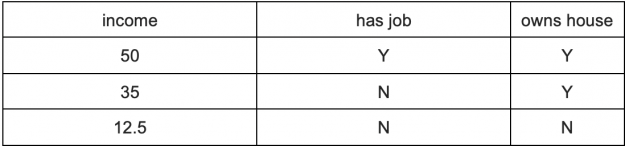
In tabular datasets, columns represent the measurements of a variable (a.k.a. feature), and rows represent individual data points. For example, the table below shows a small dataset with three columns: “has job”, “owns house” and “income”. In this example “income” is the label (sometimes known as the target variable for prediction) and the other columns are features used to try to predict the income.
Table 1: Income dataset
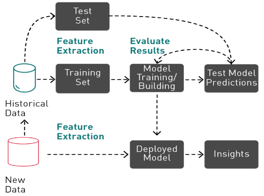
Supervised Machine learning is an iterative, exploratory process that involves Data preparation, feature engineering, validation splitting, missing value handling, training, testing, hyperparameter tuning, ensembling, and evaluating ML models before a model can be used in production to make predictions.
Figure 2: Machine learning is an iterative process involving feature extraction, training, and evaluating before a model can be deployed to make predictions.
What is AutoML
Historically, achieving state-of-the-art ML performance required extensive background knowledge, experience, and human effort. Depending on the tool and level of automation, AutoML uses different algorithmic techniques to try to find the best features, hyperparameters, algorithms, and or combination of algorithms for an ml pipeline. By automating time-consuming ML pipelines, practitioners and enterprises can apply machine learning to solve business problems faster and more easily.
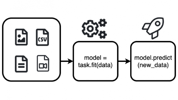
AutoML in 3 steps with AutoGluon Tabular
AutoGluon Tabular can be used to automatically build state-of-the-art models that predict a particular column’s value based on the other columns in the same row using two functions: fit (), and predict () as shown below.
from autogluon.tabular import TabularPredictor, TabularDataset
# load dataset
train_data = TabularDataset(DATASET_PATH)
# fit the model
predictor = TabularPredictor(label=LABEL_COLUMN_NAME).fit(train_data)
# make predictions on new data
prediction = predictor.predict(new_data)
Figure 3: The AutoGluon fit() function automatically builds an ML model which can be used to predict a particular column’s value based on the other columns in the same row with the predict() function.
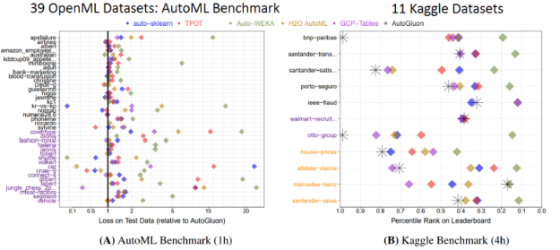
With this simple code, AutoGluon beats other AutoML frameworks and many top data scientists. An extensive evaluation with tests on a suite of 50 classification and regression tasks from Kaggle and the OpenML AutoML Benchmark revealed that AutoGluon is faster, more robust, and more accurate than TPOT, H2O, AutoWEKA, auto-sklearn, and Google AutoML Tables. Also in two popular Kaggle competitions, AutoGluon beat 99% of the participating data scientists after merely 4 hours of training on the raw data.
Figure 4: AutoGluon outperformed other AutoML frameworks and many top Kaggle data scientists.
What is different about AutoGluon?
Most AutoML frameworks focus on the task of Combined Algorithm Selection and Hyperparameter optimization (CASH), offering strategies to find the best model and its hyperparameters from a wide selection of possibilities. However, CASH has some drawbacks:
It requires many repeated model training and most of the models are thrown away without contributing to the final result.
The more hyperparameter tuning is done, the higher the risk of overfitting the validation data.
Hyperparameter tuning is less helpful when ensembling.
In contrast, AutoGluon-Tabular outperforms other frameworks by relying on methods used by expert data scientists to win competitions: ensembling multiple models and stacking them in multiple layers.
How does Ensembling Work?
Ensemble learning methods combine multiple machine learning (ML) algorithms to obtain a better model. To understand this better, let’s go over Random Forests, which is an ensemble of decision trees.
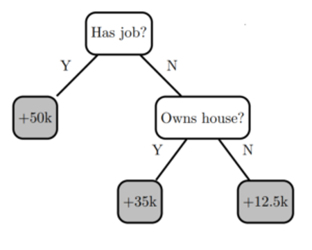
Decision trees create a model that predicts the target label by evaluating a tree of if-then-else and true/false feature questions and estimating the minimum number of questions needed to assess the probability of making a correct decision. Decision trees can be used for classification to predict a category or regression to predict a continuous numeric value. For example, the decision tree below (based on the table above) , tries to predict the label “income” using two decision nodes for the features “has job” and “owns house”.
Figure 5: A simple decision tree model with two decision nodes and three leaves.
Decision trees have the advantage that they are easy to interpret, but they have problems with overfitting and accuracy. Building an accurate model is somewhere in between underfitting and overfitting —where the model predictions match how the training data behaves and is also generalized enough to make accurate predictions on unseen data.
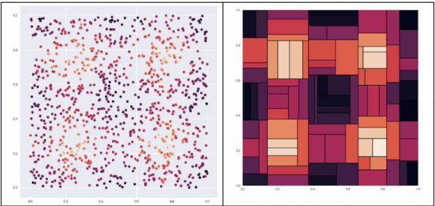
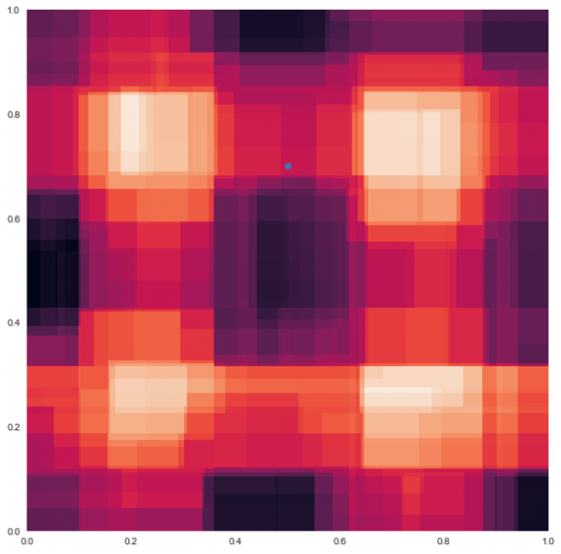
Decision trees seek to find the best split to subset the data, which results in harsh splits. For example, given the dataset below on the left we want to predict the color of a dot where the lighter the dot is the higher the value. A decision tree, shown on the right, would split the data into harsh chunks. Next we will look at how to improve on decision trees with ensembling.
Figure 6: Example dataset on the left, where the goal is to predict the color of a dot where the lighter the dot is the higher the value. The decision tree for this dataset on the right splits the data into harsh chunks.
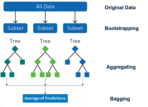
Ensembling is a proven approach to improve the accuracy of models, by combining their predictions and improving generalization. Random forest is a popular ensemble learning method for classification and regression. Random forest uses a technique called bagging (bootstrap aggregating) to build full decision trees in parallel from random bootstrap samples of the data set and features. Predictions are made by aggregating the output from all the trees, which reduces the variance and improves the predictive accuracy. The final prediction is a majority class or mean regression of all the decision tree predictions. Randomness is critical to the success of the forest, bagging makes sure that no decision trees are the same, reducing the problems of overfitting seen with individual trees.
Figure 7: Random forest uses a technique called bagging to build decision trees from random bootstrap samples of the data set and features.
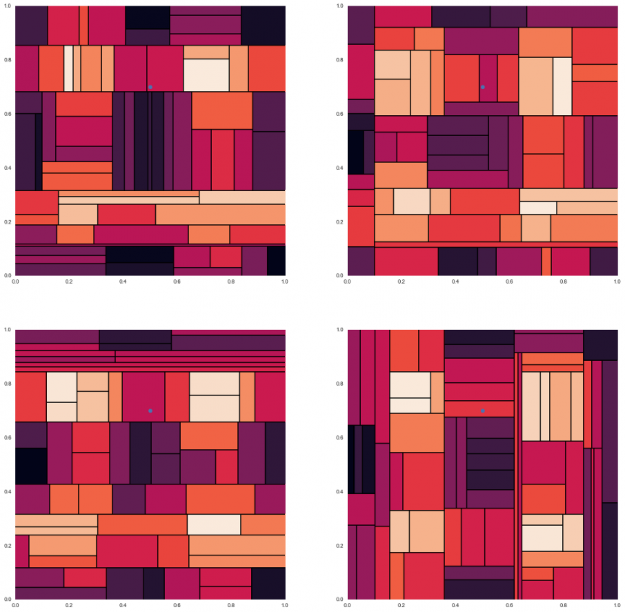
To understand how this gives better predictions, let’s look at an example. Here, are four different decision trees for the data set seen in figure 6, with different prediction colors for a test data point. We can see that each gives approximations of the solution which are not generalized enough to make accurate predictions.
Figure 8: Four different decision trees for the data set seen in figure 6, with different prediction colors for a test data point. image reference https://gist.github.com/tylerwx51/fc8b316337833c877785222d463a45b0
When these four decision trees are combined and averaged together the harsh boundaries go away and are smoothed as in the random forest example below. Now the prediction color for the test data point is a blend of the colors from the other tree predictions.
Figure 9: Random forest model for the four decision trees from figure 8.
All of the decision trees in a random forest are suboptimal, they are all wrong in random directions. When you average the decision trees, the reasons they are wrong cancel out each other, this is called variance cancellation. The results are of higher quality because they reflect decisions reached by the majority of trees. The averaging limits errors, even though some trees are wrong, others will be right, so the group of trees collectively moves in the correct direction.
When many uncorrelated decision trees are combined, they produce models with high predictive power resilient to over-fitting. These concepts are foundational to popular machine learning algorithms such as Random Forest, XGBoost, Catboost and LightGBM which are employed by AutoGluon.
Multi-layer Stack Ensembling
You can go further than this with ensembling, experienced machine learning practitioners combine outputs of RandomForest, CatBoost, k-nearest neighbors, and others to further improve model accuracy. In the ML competition community it is hard to find a competition won by a single model, every winning solution incorporates ensembles of models.
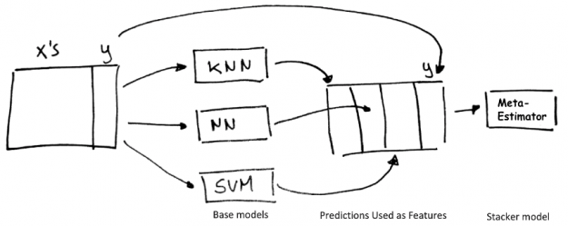
Stacking is a technique that uses the aggregated predictions of a collection of “base” regression or classification models as the features for training a meta-classifier or regressor “stacker” model.
Figure 10: Stacking technique.
Multi-layer stacking feeds the predictions output by the stacker models as inputs to additional higher layer stacker models. Iterating this process in multiple layers has been a winning strategy in many Kaggle competitions. Multi-layer stacking ensembles are powerful but difficult to use and implement robustly and are not currently utilized by any AutoML framework except Autogluon.
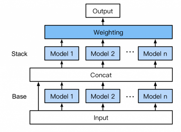
Without the need for expert knowledge, AutoGluon automatically assembles and trains a novel form of multi-layer stack ensembling with k-fold bagging shown in figure 11. Here’s how it works:
Base: the first layer has multiple base models which are individually trained and bagged using k-fold ensemble bagging (discussed below).
Concatenating: The base layer model predictions are concatenated along with the input features, to use as input for training the next layer.
Stacking: Multiple stacker models are trained on the concat layer output. Unlike traditional stacking strategies, AutoGluon reuses the same base layer model types (with the same hyperparameter values) as stackers. Also, the stacker models take as input not only the predictions of the models at the previous layer but also the original data features themselves.
Weighting: The final stacking layer applies ensemble selection to aggregate the stacker models’ predictions in a weighted manner. Aggregating predictions across a high-capacity stack of models improve resilience against over-fitting
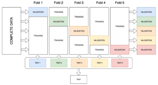
AutoGluon improves stacking performance by utilizing all of the available data for both training and validation, through k-fold ensemble bagging of all models at all layers of the stack. k-fold ensemble bagging is similar to k-fold cross validation, which is a method that maximizes the training dataset and is typically used for hyperparameter tuning to determine the best model parameters. With k-fold cross-validation, the data is randomly split into k partitions (folds). Each fold is used one time as the validation dataset, while the rest (Out-Of-Fold – OOF) are used for training. Models are trained using the OOF training sets and evaluated with the validation sets, resulting in k model accuracy measurements. Instead of determining the best model and throwing away the rest, AutoGluon bags all models and obtains OOF predictions from each model on the partition it did not see during training. This creates k-fold predictions of each model which are used as meta-features for the next layer.
Figure 12: k-fold Ensemble Bagging.
To further improve predictive accuracy and reduce overfitting, AutoGluon-Tabular repeats the k-fold bagging process on n different random partitions of the training data, averaging all OOF predictions over the repeated bags. The number n is chosen by estimating how many rounds can be completed within the specified time constraints when calling the fit() function.
Why AutoGluon Needs GPU Acceleration
Multilayer stack ensembling improves accuracy, however, this means training hundreds of models, a much more compute-intensive task than basic ML use cases, and 10 to 20 times more expensive than weighted ensembling. In the past, the complexity and computational requirements made multilayer stack ensembling difficult to implement for many production use cases and large datasets. With AutoGluon and NVIDIA GPU computing, this is no longer the case.
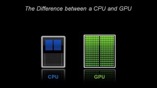
Architecturally, the CPU is composed of just a few cores with lots of cache memory that can handle a few software threads at a time. In contrast, a GPU is composed of hundreds of cores that can handle thousands of threads simultaneously. GPUs have been shown to perform over 20x faster than CPUs in ML workflows and have revolutionized the deep learning field.
Figure 13: A CPU is composed of just a few cores, in contrast, a GPU is composed of hundreds of cores.
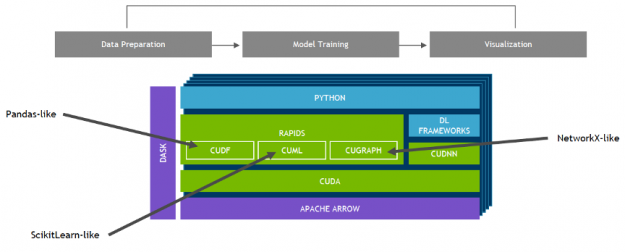
NVIDIA developed RAPIDS—an open-source data analytics and machine learning acceleration platform—for executing end-to-end data science training pipelines completely in GPUs. It relies on NVIDIA® CUDA® primitives for low-level compute optimization, but exposes that GPU parallelism and high memory bandwidth through user-friendly Python interfaces like Pandas and Scikit-Learn APIs.
With RAPIDS’s cuML, popular machine learning algorithms like random forest, XGBoost, and many others are supported for both single-GPU and large data center deployments. For large datasets, these GPU-based implementations can accelerate the training of machine learning models — by up to 45x in the case of random forests, over 100x for support vector machines, and up to 600x for k-nearest neighbors. These speedups can turn overnight jobs into interactive jobs, allow exploration of larger datasets, and enable trying dozens of model variants in the time it would have previously taken to train a single model.
Figure 14: Data science pipeline with GPUs and RAPIDS.
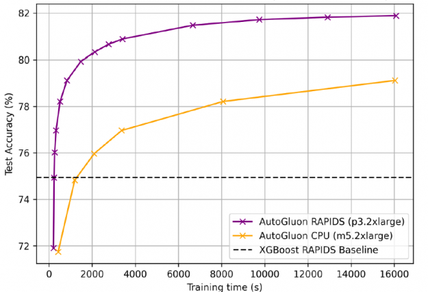
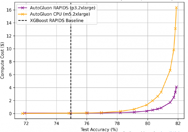
For the 115-million-row airline dataset used in the gradient boosting machines (GBM) benchmarks suite, AutoGluon + RAPIDS accelerated training by 25x compared to AutoGluon on CPUs, with 81.92% accuracy, 7% above the XGBoost baseline. GPUs prefer longer training times as fixed start up costs become less significant.
Figure 15: AutoGluon + RAPIDS accelerated training by 25x compared to AutoGluon on CPUs, with 81.92% accuracy.
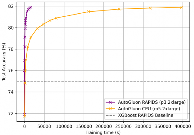
In order to obtain 81.92% accuracy, AutoGluon + RAPIDS on GPUs trained in 4 hours versus 4.5 days for CPUs.
Figure 16: AutoGluon + RAPIDS on GPUs trained in 4 hours versus 4.5 days for CPUs.
AutoGluon + RAPIDS on GPUs was not only faster, it also cost less, ¼ as much as CPUs to train to the same accuracy (AWS EC2 pricing: p3.2xlarge $0.9180/hr, m5.2xlarge $0.1480/hr).
Figure 17: AutoGluon + RAPIDS on GPUs also cost less, ¼ as much as CPUs to train to the same accuracy.
The AutoGluon website features numerous tutorials for developers to leverage machine learning for tabular, text, and image data (covering both basic tasks like classification/regression as well as more advanced tasks like object detection).
Conclusion
The AutoGluon AutoML toolkit makes it easy to train and deploy cutting-edge accurate machine learning models for complex business problems. In addition the integration of AutoGluon with RAPIDS leverages the full potential of NVIDIA GPU computing, enabling complex models to train up to 40x faster and predict 10x faster.
I would appreciate if you could give me any notes. I’m also trying to translate this to TensorFlow, but it’s not as trivial as I initially thought, considering indexing is very different (my implementation relies on selecting the multiple regions at once with `image[…, r, c]`, where `r` and `c` are two index matrices).
Any ideas on this would be greatly appreciated!
Have a great day. 🙂
The most commonly diagnosed cancer in the US today is skin cancer. There are three main variants: melanoma, basal cell carcinoma (BCC), and squamous cell carcinoma (SCC). Though melanoma only accounts for roughly 1% of all skin cancers, it is the most fatal, metastasizing rapidly without early detection and treatment. This makes early detection critical, … Continued
The most commonly diagnosed cancer in the US today is skin cancer. There are three main variants: melanoma, basal cell carcinoma (BCC), and squamous cell carcinoma (SCC). Though melanoma only accounts for roughly 1% of all skin cancers, it is the most fatal, metastasizing rapidly without early detection and treatment. This makes early detection critical, as numerous studies show significantly better survival rates when detection is done in its earliest stages.
The current diagnosis procedure is done through a visual examination by a dermatologist, followed by a biopsy to confirm any suspected pathology. This manual examination is dependent on human subjectivity and thus suffers from error at a concerning rate. When a primary care physician looks for skin cancer, their sensitivity, or ability to identify a patient with the disease correctly, is only 0.45, while a dermatologist has a sensitivity of 0.97.
In recent years, the use of deep learning to perform medical diagnostics has become a quickly growing field. In this post, we discuss developing an end-to-end example of how deep learning could lead to an automated dermatology exam system free of human bias, using the recently announced NVIDIA Clara AGX development kit.
Datasets and models
This reference application is the pairing of two deep learning models:
An object detection model (YOLOv4) that looks for moles on the body through a camera. This model was trained with an original dataset created from annotating body mole images.
A classification model (EfficientNet) that receives moles from the object detection model and then determines if it is benign, unknown, or melanoma. The classification model was trained using the SIIM-ISIC melanoma Kaggle challenge dataset.
Figure 1 shows the workflow of the algorithm using a single video frame. The application can use a high-definition webcam or IP camera as input to the models, or even run on a previously captured video.
Figure 1. Skin mole detection and classification workflow.
Clara AGX development kit
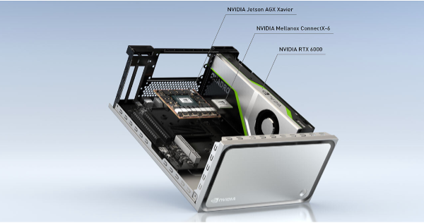
This reference application was built using the NVIDIA Clara AGX development kit, a high-end performance workstation built with medical applications in mind. The system includes an RTX 6000 GPU, delivering 200+ INT8 AI TOPs of peak performance and 24 GB of VRAM, leaving plenty of overhead for running multiple models.
Figure 2. Clara AGX Developer Kit.
In addition, the AGX platform offers support for high bandwidth sensors through 100G Ethernet and an NVIDIA ConnectX-6 network interface card (NIC). NVIDIA partners are currently using the NVIDIA Clara AGX development kit to develop applications in ultrasound, genomics, and endoscopy.
The Clara AGX Developer Kit is currently available exclusively for members of the NVIDIA Clara Developer Partner Program. After you register, we’ll be in touch.
Summary
We’ve provided a research prototype of a dermatology application, but what would it take to transform this into a real application?
Commercially usable data. The SIIM-ISIC dataset is strictly for non-commercial use.
A much larger object detection dataset. The dataset that we used consisted of only a few hundred annotated images, which did lead to a larger than desired number of false positives.
Run the models at the “speed of light” (SOL). SOL often entails training models to run using mixed precision and then transforming the models to work with the NVIDIA TensorRT framework. TensorRT is designed to optimize model inference on NVIDIA GPUs and work with common frameworks such as PyTorch and TensorFlow. These steps would help to ensure that your application pipeline runs in real-time.
FDA clearance. Any developed medical application must be cleared by the FDA. Today, there are over 70 FDA-cleared AI applications, and the FDA has been active in soliciting feedback from developers in this area. This is typically a long (18 months) and arduous process, but a necessary one.
Researchers from NVIDIA, University of Texas at Austin and Caltech developed a simple, efficient, and plug-and-play uncertainty quantification method for the 6-DoF object pose estimation task, using an ensemble of K pre-trained estimators with different architectures and/or training data sources.
Researchers from NVIDIA, University of Texas at Austin and Caltech developed a simple, efficient, and plug-and-play uncertainty quantification method for the 6-DoF (degrees of freedom) object pose estimation task, using an ensemble of K pre-trained estimators with different architectures and/or training data sources.
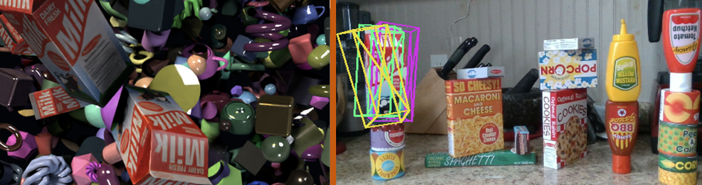
FastUQ focuses on the uncertainty quantification for deep object pose estimation. In deep learning-based object pose estimation (see NVIDIA DOPE), a big challenge is deep-learning-based pose estimators might be overconfident in their pose predictions.
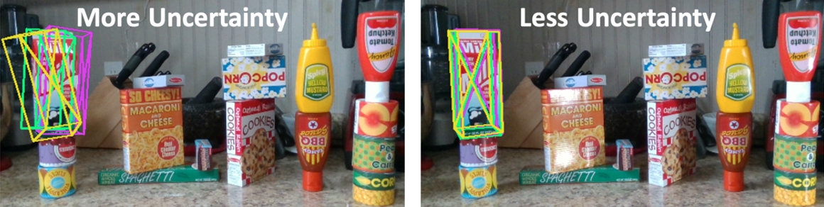
For example, the two figures below are the pose estimation results for the “Ketchup” object from a DOPE model in a manipulation task. Both results are very confident, but the left one is incorrect.
Another challenge addressed is the sim2real gap. Typically, deep learning-based pose estimators are trained from synthetic datasets (by NVIDIA’s ray tracing renderer, NViSII), but we want to apply these estimators in the real world and quantify the uncertainty. For example, the left figure is from the synthetic NViSII dataset, and the right one is from the real world.
In this project, we propose an ensemble-based method for the fast uncertainty quantification of deep learning-based pose estimators. The idea is demonstrated in the following two figures, where in the left one the deep models in the ensemble disagree with each other, which implies more uncertainty; and in the right one these models agree with each other, which reflects less uncertainty.
This research is definitely interdisciplinary and it was solved by the joint efforts of different research teams at NVIDIA:
The AI Algorithms team led by Anima Anandkumar, and the NVIDIA AI Robotics Research Lab in Seattle working on the uncertainty quantification methods
The Learning and Perception Research team led by Jan Kautz for training the deep object pose estimation models, and providing photorealistic synthetic data from NVIDIA’s ray-tracing renderer, NViSII
For training the deep estimators and generating the high-fidelity photorealistic synthetic datasets, the team used NVIDIA V100 GPUs and NVIDIA OptiX (C++/CUDA back-end) for acceleration.
FastUQ is a novel fast uncertainty quantification method for deep object pose estimation, which is efficient, plug-and-play, and supports a general class of pose estimation tasks. This research has potentially significant impacts in autonomous driving and general autonomy, including more robust and safe perception, and uncertainty-aware control and planning.
Posted by Diego Martin Arroyo, Software Engineer and Federico Tombari, Research Scientist, Google Research
Information in a written document is not only conveyed by the meaning of the words contained in it, but also by the overall document layout. Layouts are commonly used to direct the order in which the reader parses a document to enable a better understanding (e.g., with columns or paragraphs), to provide helpful summaries (e.g., with titles) or for aesthetic purposes (e.g., when displaying advertisements).
While these design rules are easy to follow, it is difficult to explicitly define them without quickly needing to include exceptions or encountering ambiguous cases. This makes the automation of document design difficult, as any system with a hardcoded set of production rules will either be overly simplistic and thus incapable of producing original layouts (causing a lack of diversity in the layout of synthesized data), or too complex, with a large set of rules and their accompanying exceptions. In an attempt to solve this challenge, some haveproposed machine learning (ML) techniques to synthesize document layouts. However, most ML-based solutions for automatic document design do not scale to a large number of layout components, or they rely on additional information for training, such as the relationships between the different components of a document.
In “Variational Transformer Networks for Layout Generation”, to be presented at CVPR 2021, we create a document layout generation system that scales to an arbitrarily large number of elements and does not require any additional information to capture the relationships between design elements. We use self-attention layers as building blocks of a variational autoencoder (VAE), which is able to model document layout design rules as a distribution, rather than using a set of predetermined heuristics, increasing the diversity of the generated layouts. The resulting Variational Transformer Network (VTN) model is able to extract meaningful relationships between the layout elements (paragraphs, tables, images, etc.), resulting in realistic synthetic documents (e.g., better alignment and margins). We show the effectiveness of this combination across different domains, such as scientific papers, UI layouts, and even furniture arrangements.
VAEs for Layout Generation The ultimate goal of this system is to infer the design rules for a given type of layout from a collection of examples. If one considers these design rules as the distribution underlying the data, it is possible to use probabilistic models to discover it. We propose doing this with a VAE (widely used for tasks like image generation or anomaly detection), an autoencoder architecture that consists of two distinct subparts, the encoder and decoder. The encoder learns to compress the input to fewer dimensions, retaining only the necessary information to reconstruct the input, while the decoder learns to undo this operation. The compressed representation (also called the bottleneck) can be forced to behave like a known distribution (e.g., a uniform Gaussian). Feeding samples from this a priori distribution to the decoder segment of the network results in outputs similar to the training data.
An additional advantage of the VAE formulation is that it is agnostic to the type of operations used to implement the encoder and decoder segments. As such, we use self-attention layers (typically seen in Transformer architectures) to automatically capture the influence that each layout element has over the rest.
Transformers use self-attention layers to model long, sequenced relationships, often applied to an array of natural language understanding tasks, such as translation and summarization, as well as beyond the language domain in object detection or document layout understanding tasks. The self-attention operation relates every element in a sequence to every other and determines how they influence each other. This property is ideal to model relationships across different elements in a layout without the need for explicit annotations.
In order to synthesize new samples from these relationships, some approaches for layout generation [e.g., 1] and even for other domains [e.g., 2, 3] rely on greedy search algorithms, such as beam search, nucleus sampling or top-k sampling. Since these strategies are often based on exploration rules that tend to favor the most likely outcome at every step, the diversity of the generated samples is not guaranteed. However, by combining self-attention with the VAE’s probabilistic techniques, the model is able to directly learn a distribution from which it can extract new elements.
Modeling the Variational Bottleneck The bottleneck of a VAE is commonly modeled as a vector representing the input. Since self-attention layers are a sequence-to-sequence architecture, i.e., a sequence of n input elements is mapped onto n output elements, the standard VAE formulation is difficult to apply. Inspired by BERT, we append an auxiliary token to the beginning of the sequence and treat it as the autoencoder bottleneck vector z. During training, the vector associated with this token is the only piece of information passed to the decoder, so the encoder needs to learn how to compress the entire document information in this vector. The decoder then learns to infer the number of elements in the document as well as the locations of each element in the input sequence from this vector alone. This strategy allows us to use standard techniques to regularize the bottleneck, such as the KL divergence.
Decoding In order to synthesize documents with varying numbers of elements, the network needs to model sequences of arbitrary length, which is not trivial. While self-attention enables the encoder to adapt automatically to any number of elements, the decoder segment does not know the number of elements in advance. We overcome this issue by decoding sequences in an autoregressive way — at every step, the decoder produces an element, which is concatenated to the previously decoded elements (starting with the bottleneck vector z as input), until a special stop element is produced.
A visualization of our proposed architecture
Turning Layouts into Input Data A document is often composed of several design elements, such as paragraphs, tables, images, titles, footnotes, etc. In terms of design, layout elements are often represented by the coordinates of their enclosing bounding boxes. To make this information easily digestible for a neural network, we define each element with four variables (x, y, width, height), representing the element’s location on the page (x, y) and size (width, height).
Results We evaluate the performance of the VTN following two criteria: layout quality and layout diversity. We train the model on publicly available document datasets, such as PubLayNet, a collection of scientific papers with layout annotations, and evaluate the quality of generated layouts by quantifying the amount of overlap and alignment between elements. We measure how well the synthetic layouts resemble the training distribution using the Wasserstein distance over the distributions of element classes (e.g., paragraphs, images, etc.) and bounding boxes. In order to capture the layout diversity, we find the most similar real sample for each generated document using the DocSim metric, where a higher number of unique matches to the real data indicates a more diverse outcome.
We compare the VTN approach to previous works like LayoutVAE and Gupta et al. The former is a VAE-based formulation with an LSTM backbone, whereas Gupta et al. use a self-attention mechanism similar to ours, combined with standard search strategies (beam search). The results below show that LayoutVAE struggles to comply with design rules, like strict alignments, as in the case of PubLayNet. Thanks to the self-attention operation, Gupta et al. can model these constraints much more effectively, but the usage of beam search affects the diversity of the results.
IoU
Overlap
Alignment
Wasserstein Class ↓
Wasserstein Box ↓
# Unique Matches ↑
LayoutVAE
0.171
0.321
0.472
–
0.045
241
Gupta et al.
0.039
0.006
0.361
0.018
0.012
546
VTN
0.031
0.017
0.347
0.022
0.012
697
Real Data
0.048
0.007
0.353
–
–
–
Results on PubLayNet. Down arrows (↓) indicate that a lower score is better, whereas up arrows (↑) indicate higher is better.
We also explore the ability of our approach to learn design rules in other domains, such as Android UIs (RICO), natural scenes (COCO) and indoor scenes (SUN RGB-D). Our method effectively learns the design rules of these datasets and produces synthetic layouts of similar quality as the current state of the art and a higher degree of diversity.
IoU
Overlap
Alignment
Wasserstein Class ↓
Wasserstein Box ↓
# Unique Matches ↑
LayoutVAE
0.193
0.400
0.416
–
0.045
496
Gupta et al.
0.086
0.145
0.366
0.004
0.023
604
VTN
0.115
0.165
0.373
0.007
0.018
680
Real Data
0.084
0.175
0.410
–
–
–
Results on RICO. Down arrows (↓) indicate that a lower score is better, whereas up arrows (↑) indicate higher is better.
IoU
Overlap
Alignment
Wasserstein Class ↓
Wasserstein Box ↓
# Unique Matches ↑
LayoutVAE
0.325
2.819
0.246
–
0.062
700
Gupta et al.
0.194
1.709
0.334
0.001
0.016
601
VTN
0.197
2.384
0.330
0.0005
0.013
776
Real Data
0.192
1.724
0.347
–
–
–
Results for COCO. Down arrows (↓) indicate that a lower score is better, whereas up arrows (↑) indicate higher is better.
Below are some examples of layouts produced by our method compared to existing methods. The design rules learned by the network (location, margins, alignment) resemble those of the original data and show a high degree of variability.
LayoutVAE
Gupta et al.
VTN
Qualitative results of our method on PubLayNet compared to existing state-of-the-art methods.
Conclusion In this work we show the feasibility of using self-attention as part of the VAE formulation. We validate the effectiveness of this approach for layout generation, achieving state-of-the-art performance on various datasets and across different tasks. Our research paper also explores alternative architectures for the integration of self-attention and VAEs, exploring non-autoregressive decoding strategies and different types of priors, and analyzes advantages and disadvantages. The layouts produced by our method can help to create synthetic training data for downstream tasks, such as document parsing or automating graphic design tasks. We hope that this work provides a foundation for continued research in this area, as many subproblems are still not completely solved, such as how to suggest styles for the elements in the layout (text font, which image to choose, etc.) or how to reduce the amount of training data necessary for the model to generalize.
AcknowledgementsWe thank our co-author Janis Postels, as well as Alessio Tonioni and Luca Prasso for helping with the design of several of our experiments. We also thank Tom Small for his help creating the animations for this post.
NVIDIA RTX ray tracing has transformed graphics and rendering. With powerful software applications like Luxion KeyShot, more users can take advantage of RTX technology to speed up graphic workflows — like rendering caustics.
NVIDIA RTX ray tracing has transformed graphics and rendering. With powerful software applications like Luxion KeyShot, more users can take advantage of RTX technology to speed up graphic workflows — like rendering caustics.
Caustics are formed as light refracts through or reflects off specular surfaces. Examples of caustics include the light focusing through a glass, the shimmering light at the bottom of a swimming pool, and even the beams of light from windows into a dusty environment.
When it comes to rendering caustics, photon mapping is an important factor. Photon mapping works by tracing photons from the light sources into the scene and storing these photons as they interact with the surfaces or volumes in the scene.
KeyShot implements a full progressive photon-mapping algorithm on the GPU that’s capable of rendering caustics, including reflections of caustics.
With the combination of RTX technology and CUDA programming framework, it is now possible for users to achieve features like ray tracing, photon mapping, and shading running on the GPU. The power of the RTX GPUs accelerates full rendering of caustics, resulting in detailed, interactive images with reflections and refractions.
Image courtesy of David Merz III at Vyzdom.
When developing KeyShot 10, the team analyzed the GPU implementation and decided to see if they could improve the photon map implementation and obtain faster caustics. The result is a caustics algorithm that is able to handle thousands of lights, quickly render highly detailed caustics up close, and run significantly faster on the new NVIDIA Ampere RTX GPUs.
“Using the new caustics algorithm in KeyShot 10, we started getting details and fine structures in the caustics that normally would not be seen due to the time it takes to get to this detail level”, said Dr. Henrik Wann Jensen, chief scientist at Luxion.
All images are rendered on the GPU and they can all be manipulated interactively in KeyShot 10 and the caustics updates with any changes made to the scene.
Image courtesy of David Merz III at Vyzdom.
“The additional memory in NVIDIA RTX A6000 is exactly what I need for working with geometry nodes in KeyShot, and I even tested how high I could push the VRAM with the ice cube scene,” said David Merz, founder and chief creative at Vyzdom. “I’m hooked on the GDDR6 memory, and I could definitely get used to this 48GB ceiling. Not needing to worry about VRAM limitations allows me to get into a carefree creative rhythm, turning a process from frustrating to fluid artistic execution, which benefits both the client and me”.
With NVIDIA RTX GPUs powering caustics algorithms in KeyShot 10, users working with transparent or reflective products can easily render high-quality images with photorealistic details.

 NVIDIA SimNet is a physics-informed neural network (PINNs) toolkit, which addresses these challenges using AI and physics.
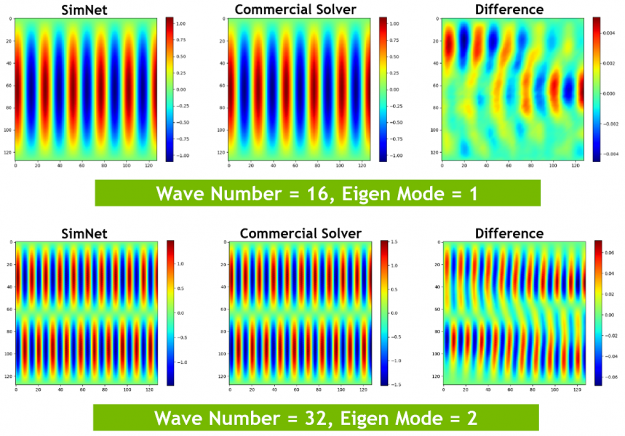
 To achieve state-of-the-art machine learning (ML) solutions, data scientists often build complex ML models. However, these techniques are computationally expensive, and until recently required extensive background knowledge, experience, and human effort. Recently, at GTC21, AWS Senior Data Scientist Nick Erickson gave a session sharing how the combination of AutoGluon, RAPIDS, and NVIDIA GPU computing simplifies …

")
 The most commonly diagnosed cancer in the US today is skin cancer. There are three main variants: melanoma, basal cell carcinoma (BCC), and squamous cell carcinoma (SCC). Though melanoma only accounts for roughly 1% of all skin cancers, it is the most fatal, metastasizing rapidly without early detection and treatment. This makes early detection critical, …
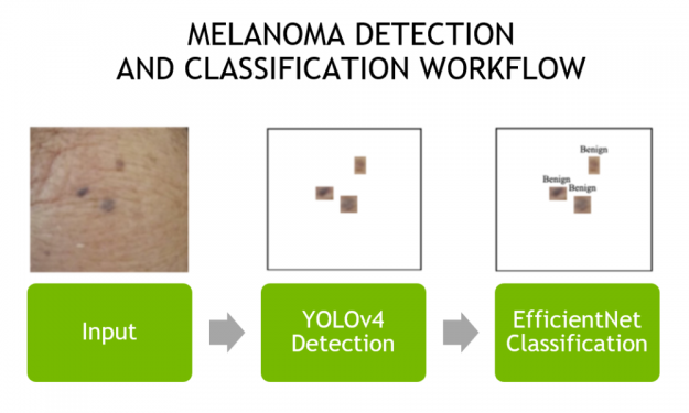
 Researchers from NVIDIA, University of Texas at Austin and Caltech developed a simple, efficient, and plug-and-play uncertainty quantification method for the 6-DoF object pose estimation task, using an ensemble of K pre-trained estimators with different architectures and/or training data sources.
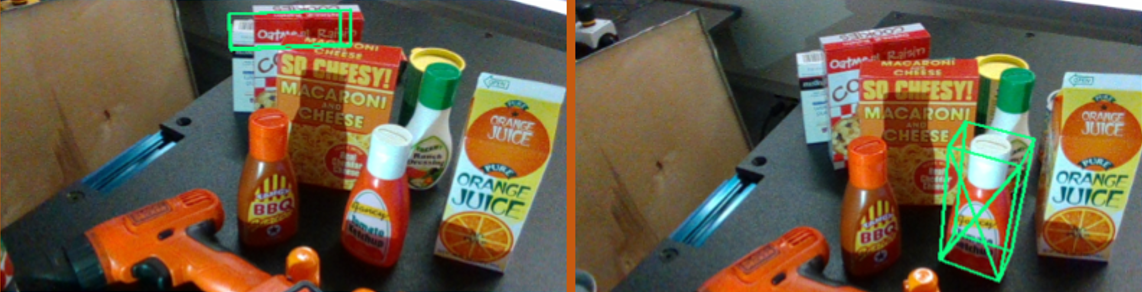


 NVIDIA RTX ray tracing has transformed graphics and rendering. With powerful software applications like Luxion KeyShot, more users can take advantage of RTX technology to speed up graphic workflows — like rendering caustics.