Use the high-level nvCOMP API for easy compression and decompression and the low-level API for more advanced workflows.
Compression can improve performance in a variety of use cases such as DL workloads, databases, and general HPC. On the GPU, compression can accelerate inter-GPU communications for collaborative workflows. It can increase the size of datasets that a single GPU can handle by compressing data before it’s stored to global memory. It can also accelerate the data link between the CPU and GPU.
For any of these workflows to be beneficial, compression and decompression must be fast and operate at a high enough compression ratio on a given dataset to be useful. However, compression ratios and throughputs of different algorithms vary widely from dataset to dataset. It can be difficult to select the best one without a lot of specialized knowledge about the algorithms and data statistics.
The NVIDIA nvCOMP library enables you to incorporate high-performance GPU compression and decompression in your applications. The library provides a set of unified APIs that allow you to quickly swap compression formats to achieve best performance on your datasets with minimal changes to code.
With nvCOMP, you can quickly and easily experiment with different algorithms to find the one with the best performance for your use case. In recent releases, we’ve updated nvCOMP to further improve and unify the interfaces. As of the newly released version 2.2, we provide an easy-to-use, high-level C++ API and a versatile low-level batch C API. In this post, we cover both interfaces in detail. You also learn how to use them effectively and when you should choose one over the other.
High-level API
The high-level API is easier to use and abstracts the work of exposing parallelism to the GPU. It is most useful when you have to compress a contiguous buffer into a contiguous, compressed buffer. This works well, for example, when compressing a buffer before sending it over a network or saving it to disk.
The following examples use the high throughput GDeflate compression format. GDeflate is deflate-like and can be mapped efficiently to data parallel architectures, such as GPUs. It is a good starting point if you that don’t have constraints on the compression format to use.
The high-level interface is a C++ API based on the nvcompManagerBase class hierarchy. Each derived Manager class is declared in its associated header in nvcomp/include. For example, the GDeflateManager used in this post is declared in nvcomp/include/gdeflate.hpp.
To get started, construct the desired Manager class. Each Manager constructor has a unique set of arguments; however, a few arguments are generally shared. All subclasses allow construction with a specified stream ID to use for all kernels and memory transfers. You can also specify the device ID to use. If you don’t specify values for these two arguments, the default stream and device are used.
Another common input is the uncompressed chunk size. This is used during compression to split the buffer into independent chunks for processing. Larger chunk sizes typically lead to higher compression ratios at the expense of less parallelism exposed to the GPU. A good starting chunk size is 64 KB, but feel free to experiment with these values to explore the associated tradeoffs for your datasets.
The Manager classes are also constructed with format-specific arguments. You can check the associated header in nvcomp/include for a description of the arguments to the Manager class constructor and to see how to construct the Manager object for your chosen format.
const size_t uncomp_chunk_size = 64 * 1024;

cudaStream_t stream;
cudaStreamCreate(&stream));
const int gdeflate_algorithm = 0; // Use standard GDeflate
const int device_id = 0; // Use the default device

GdeflateManager gdeflate_manager{chunk_size, gdeflate_algorithm, stream, device_id};
nvcompManager requires a temporary scratch workspace to do compression and decompression. This required scratch space is of fixed size based on the particular compression format arguments and the maximum occupancy of the compression and decompression kernels. If it makes sense for your use case, you can provide a scratch buffer to the nvcompManager object after construction, using set_scratch_buffer.
Manually setting the scratch buffer may be desirable to control the memory allocation scheme used for this allocation. If you’re OK with the default, we suggest skipping this step and enabling the nvcompManager object to handle the allocation.
This buffer is reused for all compression and decompression operations that nvcompManager performs. If the nvcompManager object allocates the scratch buffer, it is freed when the object is destroyed.
Compression
Now you’re ready to compress a buffer. First, configure the compression using the configure_compression API. This asynchronous operation returns a CompressionConfig object.
The configuration step only requires the size of the input-uncompressed buffer. You must allocate a GPU-accessible memory buffer of at least this size to serve as the result buffer for the compression routine. With this information, compression can be performed, as shown in the following code example:
The buffer that results from high-level interface compression includes a header before the compressed data (Figure 1). This header includes information about how the buffer was compressed, so that you can construct an nvcompManager object from a compressed buffer without knowing how it was compressed. This enables you to decompress a buffer without knowing how it was compressed.
Figure 1. HLIF compressed data format
To do this, use the create_manager API declared in nvcompManagerFactory.hpp. This synchronous API takes as input the compressed buffer along with optional stream and device IDs.
auto decomp_nvcomp_manager = create_manager(comp_buffer, stream);
If you already have the information about how the buffer was compressed, you can construct a new manager using that configuration as described earlier. You can also reuse the same nvcompManager object that was used for compression to perform decompression. These approaches have the advantage that they don’t require synchronizing the stream.
Given an nvcompManager object and a compressed buffer, decompression is performed similarly to compression with a couple of minor differences. For one, there are two possible ways to do the decompression configuration. If you have the CompressionConfig object used for the compression, you can configure the decompression completely asynchronously.
One example use case for this API is in the training of large neural networks. The size of the neural network or the size of the training set that you can use is limited based on the memory capacity of the GPU. Using compression, you can effectively increase this capacity without having to offload data to the CPU or use multiple GPUs.
Specifically, backpropagation-based training involves computing activation maps during the forward pass and then reusing them in the computation of the backward pass. These activation maps are large and relatively sparse, making them good fits for compression. Use the gdeflate_manager to compress the maps and hold in memory the compressed buffers and the CompressionConfig objects from each layer of the network. This enables fully asynchronous backpropagation, including decompression.
You can also configure the decompression using the compressed buffer if you don’t have the CompressionConfig object that was used. This is a synchronous operation that must perform a cudaMemcpyAsync operation from the device. All synchronization is on the stream specified in the nvcompManager constructor and is not device-wide.
Finally, there are two types of error checking in the high-level API: std::runtime_error exceptions and checking the nvcompStatus_t value.
If any CUDA APIs fail, these raise std::runtime_error exceptions. You can catch these in your application or leave them unhandled, in which case your application fails with a descriptive error message of what went wrong. This can happen if, for example, the output buffer that you provided was of insufficient size or wasn’t accessible on the GPU.
The second form of error-checking is to check the nvcompStatus_t value in the CompressionConfig or DecompressionConfig object. This status is set during the associated kernel call. Corrupt input buffers and other errors trigger it.
Low-level API
The low-level API provides a C API for more advanced workflows. The low-level API simultaneously compresses and decompresses batches of independent chunks that you provided. It’s up to you to chunk the data and to provide a sufficient number of chunks to exploit the GPU’s parallel processing capabilities.
This is the most efficient way to process the data if you have many independent, discontiguous buffers. The low-level API avoids the workload of packing the resulting compressed chunks into a single contiguous-compressed buffer. It also avoids the compression ratio overhead associated with saving information about how the buffer was compressed as in the high-level API.
This workflow fits well with database applications, for example, where you tend to have many independent columns to compress or decompress. This API is used in RAPIDS and in the NVIDIA Spark implementation.
Compression
For compression in the low-level API, you must allocate a temporary scratch buffer. The temporary buffer is similar to that described in the high-level API. However, the buffer size is dependent on the size of the input buffer so it must be redefined and possibly reallocated with each new set of user inputs.
Next, the maximum size of a compressed chunk in the batch should be computed. This allows you to allocate a collection of result buffers. In the following example, batch_size is the number of chunks to process. The device array of result pointers is constructed in pinned host memory before copying to the device.
size_t max_out_bytes;
nvcompBatchedGdeflateCompressGetMaxOutputChunkSize(chunk_size, nvcompBatchedGdeflateDefaultOpts, &max_out_bytes);
// Allocate output space on the device
void ** host_compressed_ptrs;
cudaMallocHost((void**)&host_compressed_ptrs, sizeof(size_t) * batch_size);
for(size_t ix_chunk = 0; ix_chunk
With all these inputs computed, you can now do compression asynchronously as shown.
To begin work towards decompression, pre-compute the decompressed sizes based on the compressed buffer. If you already have this information, skip this step.
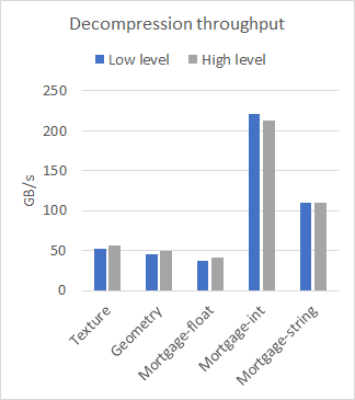
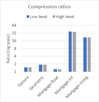
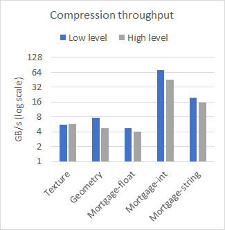
nvCOMP provides a set of benchmarks for each of the formats in the low-level and high-level format. Figure 2 compares the performance of high-level and low-level on a few different datasets, with large contiguous buffers. The results were collected using the A100 GPU.
Figure 2a. Decompression throughputs for various datasets.Figure 2b. Compression ratios for various datasets.Figure 2c. Compression throughputs for various datasets
As you can see from the results, the difference in performance between the low– and high-level APIs is negligible when working with large contiguous buffers. The choice of which to use then comes down to your use case. Use the low-level API if you have many small buffers or to avoid the memory footprint associated with the high-level API.
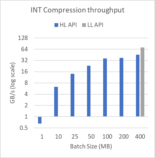
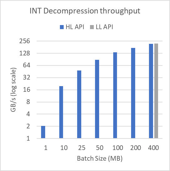
Figure 3 shows performance across different buffer sizes in log-scale. To produce these results, the mortgage-int dataset presented as part of Figure 2 was split into many batches of batchSize as shown. The file is over 314 MB. For the 1 MB batch size, 315 compression and decompression operations are performed. At a 400 MB batch size, a single compression and decompression operation is performed.
Batching the data in this way doesn’t affect the low-level batch API.
Figure 3a: Compression throughputs for various batch sizes operating on a 314 MB file.Decompression throughputs for various batch sizes operating on a 314 MB file.
As demonstrated, the performance of the high-level interface degrades heavily for small batch sizes. This shows the utility of using the low-level batch API when compressing or decompressing many smaller buffers. The low-level batch API can do the operations using fewer, higher-occupancy kernels, while the high-level API requires many small kernel launches with associated tail effects and occupancy concerns.
We include benchmark applications with the library so that you can try out different compression formats and see which works best on your data. The provided benchmarks are benchmark_hlif and benchmark__chunked. For more information, see the nvCOMP README.
Summary
Now you’ve learned how to use the high-level nvCOMP API for easy compression and decompression. You’ve learned when it may be better to use the low-level API as well as how to use it.
For more information, see the latest version of the NVIDIA/nvcomp GitHub repo. For fully worked, compilable examples that you can adapt to your use cases, see the lowlevel_c_quickstart.md and highlevel_cpp_quickstart.md walkthroughs along with the associated example files.
this is an NLP and python based project we are trying to achieve something new this project is almost there but the only file connecting thing is leftover😌
hey everyone so i have been experimenting with object detection using python,opencv and tensorflow but i keep getting this error P.S both the code an “myData” are in the same folder
the code:
import numpy as np import matplotlib.pyplot as plt from keras.models import Sequential from keras.layers import Dense from tensorflow.keras.optimizers import Adam from keras.utils.np_utils import to_categorical from keras.layers import Dropout, Flatten from keras.layers.convolutional import Conv2D, MaxPooling2D import cv2 from sklearn.model_selection import train_test_split import pickle import os import pandas as pd import random from keras.preprocessing.image import ImageDataGenerator
########### Parameters
path = “myData” # folder with all the class folders labelFile = ‘labels.csv’ # file with all names of classes batch_size_val = 50 # how many to process together steps_per_epoch_val = 2000 epochs_val = 10 imageDimesions = (32, 32, 3) testRatio = 0.2 # if 1000 images split will 200 for testing validationRatio = 0.2 # if 1000 images 20% of remaining 800 will be 160 for validation
X_train = ARRAY OF IMAGES TO TRAIN y_train = CORRESPONDING CLASS ID ######################### TO CHECK IF NUMBER OF IMAGES MATCHES TO NUMBER OF LABELS FOR EACH DATA SET
print(“Data Shapes”) print(“Train”, end=””); print(X_train.shape, y_train.shape) print(“Validation”, end=””); print(X_validation.shape, y_validation.shape) print(“Test”, end=””); print(X_test.shape, y_test.shape) assert (X_train.shape[0] == y_train.shape[ 0]), “The number of images in not equal to the number of lables in training set” assert (X_validation.shape[0] == y_validation.shape[ 0]), “The number of images in not equal to the number of lables in validation set” assert (X_test.shape[0] == y_test.shape[0]), “The number of images in not equal to the number of lables in test set” assert (X_train.shape[1:] == (imageDimesions)), ” The dimesions of the Training images are wrong ” assert (X_validation.shape[1:] == (imageDimesions)), ” The dimesionas of the Validation images are wrong ” assert (X_test.shape[1:] == (imageDimesions)), ” The dimesionas of the Test images are wrong”
######################### READ CSV FILE
data = pd.read_csv(labelFile) print(“data shape “, data.shape, type(data))
######################### DISPLAY SOME SAMPLES IMAGES OF ALL THE CLASSES
num_of_samples = [] cols = 5 num_classes = noOfClasses fig, axs = plt.subplots(nrows=num_classes, ncols=cols, figsize=(5, 300)) fig.tight_layout() for i in range(cols): for j, row in data.iterrows(): x_selected = X_train[y_train == j] axs[j][i].imshow(x_selected[random.randint(0, len(x_selected) – 1), :, :], cmap=plt.get_cmap(“gray”)) axs[j][i].axis(“off”) if i == 2: axs[j][i].set_title(str(j) + “-” + row[“Name”]) num_of_samples.append(len(x_selected))
######################### DISPLAY A BAR CHART SHOWING NO OF SAMPLES FOR EACH CATEGORY
print(num_of_samples) plt.figure(figsize=(12, 4)) plt.bar(range(0, num_classes), num_of_samples) plt.title(“Distribution of the training dataset”) plt.xlabel(“Class number”) plt.ylabel(“Number of images”) plt.show()
######################### PREPROCESSING THE IMAGES
def preprocessing(img): img = grayscale(img) # CONVERT TO GRAYSCALE img = equalize(img) # STANDARDIZE THE LIGHTING IN AN IMAGE img = img / 255 # TO NORMALIZE VALUES BETWEEN 0 AND 1 INSTEAD OF 0 TO 255 return img
X_train = np.array(list(map(preprocessing, X_train))) # TO IRETATE AND PREPROCESS ALL IMAGES X_validation = np.array(list(map(preprocessing, X_validation))) X_test = np.array(list(map(preprocessing, X_test))) cv2.imshow(“GrayScale Images”, X_train[random.randint(0, len(X_train) – 1)]) # TO CHECK IF THE TRAINING IS DONE PROPERLY
######################### AUGMENTATAION OF IMAGES: TO MAKEIT MORE GENERIC
dataGen = ImageDataGenerator(width_shift_range=0.1, # 0.1 = 10% IF MORE THAN 1 E.G 10 THEN IT REFFERS TO NO. OF PIXELS EG 10 PIXELS height_shift_range=0.1, zoom_range=0.2, # 0.2 MEANS CAN GO FROM 0.8 TO 1.2 shear_range=0.1, # MAGNITUDE OF SHEAR ANGLE rotation_range=10) # DEGREES dataGen.fit(X_train) batches = dataGen.flow(X_train, y_train, batch_size=20) # REQUESTING DATA GENRATOR TO GENERATE IMAGES BATCH SIZE = NO. OF IMAGES CREAED EACH TIME ITS CALLED X_batch, y_batch = next(batches)
NVIDIA’s GTC conference is packed with smart people and programming. The virtual gathering — which takes place from March 21-24 — sits at the intersection of some of the fastest-moving technologies of our time. It features a lineup of speakers from every corner of industry, academia and research who are ready to paint a high-definition Read article >
I finished reading the new book on TinyML— The Tiny ML Cookbook that has just been released. Whether you are a professional seeking to dive deeper into the world of TinyML, or just starting out, you will find this book useful for your practical experiments.
I would like to share my impressions of this book with you and give you a list of similar books on this subject. This book is focused on practical TinyML use cases, which are referred to as “recipes”. The author is Gian Marco Iodice, a team and tech lead in the Machine Learning Group at Arm, who co-created the Arm Compute Library in 2017, which is currently the most performant library for ML on Arm, and it’s deployed on billions of devices worldwide.
Summarizing, it is worth mentioning the top three takeaways from this book:
Practicing the whole workflow to develop ML models for microcontroller
Learning techniques to build tiny ML models for memory-constrained devices
Developing a complete and memory-efficient vision recognition pipeline for microcontrollers
This book touches upon many use cases that will allow you to start developing machine learning applications on microcontrollers through practical examples quickly without any prior knowledge of edge devices.
The TinyML Cookbook gives a comprehensive overview of the Tiny ML applications, covering some of the essentials for developing intelligent apps on the Arduino Nano 33 BLE Sense and Raspberry Pi Pico, as well as general requirements for a good dataset. Most importantly, the book contains many examples of code and datasets ready to be deployed on any device.
Here is one thing that I find particularly useful for myself. I have been facing particular challenges in implementing an LED status indicator on the breadboard. In the past, I used to physically link two or more metal connections together when connecting external components to the microcontroller. Because of the small area between each pin, making direct contact with the microcontroller’s pins might be difficult.To make this operation run smoothly, the author provided links to the Arduino Nano and Raspberry Pi Pico pinout diagrams, offering step-by-step instructions for constructing the circuit that will turn the LED on when the platform is plugged into power. He also suggested using a new Digikey online tool to identify the color bands of the resistor.
I think it will also be useful to mention here the top five books on TinyML that I found relevant to this topic.
Posted by Amir Yazdanbakhsh, Research Scientist and Aviral Kumar, Student Researcher, Google Research
Advances in machine learning (ML) often come with advances in hardware and computing systems. For example, the growth of ML-based approaches in solving various problems in vision and language has led to the development of application-specific hardware accelerators (e.g., Google TPUs and Edge TPUs). While promising, standardprocedures for designing accelerators customized towards a target application require manual effort to devise a reasonably accurate simulator of hardware, followed by performing many time-intensive simulations to optimize the desired objective (e.g., optimizing for low power usage or latency when running a particular application). This involves identifying the right balance between total amount of compute and memory resources and communication bandwidth under various design constraints, such as the requirement to meet an upper bound on chip area usage and peak power. However, designing accelerators that meet these design constraints is often result in infeasibledesigns. To address these challenges, we ask: “Is it possible to train an expressive deep neural network model on large amounts of existing accelerator data and then use the learned model to architect future generations of specialized accelerators, eliminating the need for computationally expensive hardware simulations?”
In “Data-Driven Offline Optimization for Architecting Hardware Accelerators”, accepted at ICLR 2022, we introduce PRIME, an approach focused on architecting accelerators based on data-driven optimization that only utilizes existing logged data (e.g., data leftover from traditional accelerator design efforts), consisting of accelerator designs and their corresponding performance metrics (e.g., latency, power, etc) to architect hardware accelerators without any further hardware simulation. This alleviates the need to run time-consuming simulations and enables reuse of data from past experiments, even when the set of target applications changes (e.g., an ML model for vision, language, or other objective), and even for unseen but related applications to the training set, in a zero-shot fashion. PRIME can be trained on data from prior simulations, a database of actually fabricated accelerators, and also a database of infeasible or failed accelerator designs1. This approach for architecting accelerators — tailored towards both single- and multi-applications — improves performance upon state-of-the-art simulation-driven methods by about 1.2x-1.5x, while considerably reducing the required total simulation time by 93% and 99%, respectively. PRIME also architects effective accelerators for unseen applications in a zero-shot setting, outperforming simulation-based methods by 1.26x.
PRIME uses logged accelerator data, consisting of both feasible and infeasible accelerators, to train a conservative model, which is used to design accelerators while meeting design constraints. PRIME architects accelerators with up to 1.5x smaller latency, while reducing the required hardware simulation time by up to 99%.
The PRIME Approach for Architecting Accelerators Perhaps the simplest possible way to use a database of previously designed accelerators for hardware design is to use supervised machine learning to train a prediction model that can predict the performance objective for a given accelerator as input. Then, one could potentially design new accelerators by optimizing the performance output of this learned model with respect to the input accelerator design. Such an approach is known as model-based optimization. However, this simple approach has a key limitation: it assumes that the prediction model can accurately predict the cost for every accelerator that we might encounter during optimization! It is well established that most prediction models trained via supervised learning misclassify adversarial examples that “fool” the learned model into predicting incorrect values. Similarly, it has been shown that even optimizing the output of a supervised model finds adversarialexamples that look promising under the learned model2, but perform terribly under the ground truth objective.
To address this limitation, PRIME learns a robust prediction model that is not prone to being fooled by adversarial examples (that we will describe shortly), which would be otherwise found during optimization. One can then simply optimize this model using any standard optimizer to architect simulators. More importantly, unlike prior methods, PRIME can also utilize existing databases of infeasible accelerators to learn what not to design. This is done by augmenting the supervised training of the learned model with additional loss terms that specifically penalize the value of the learned model on the infeasible accelerator designs and adversarial examples during training. This approach resembles a form of adversarial training.
In principle, one of the central benefits of a data-driven approach is that it should enable learning highly expressive and generalist models of the optimization objective that generalize over target applications, while also potentially being effective for new unseen applications for which a designer has never attempted to optimize accelerators. To train PRIME so that it generalizes to unseen applications, we modify the learned model to be conditioned on a context vector that identifies a given neural net application we wish to accelerate (as we discuss in our experiments below, we choose to use high-level features of the target application: such as number of feed-forward layers, number of convolutional layers, total parameters, etc. to serve as the context), and train a single, large model on accelerator data for all applications designers have seen so far. As we will discuss below in our results, this contextual modification of PRIME enables it to optimize accelerators both for multiple, simultaneous applications and new unseen applications in a zero-shot fashion.
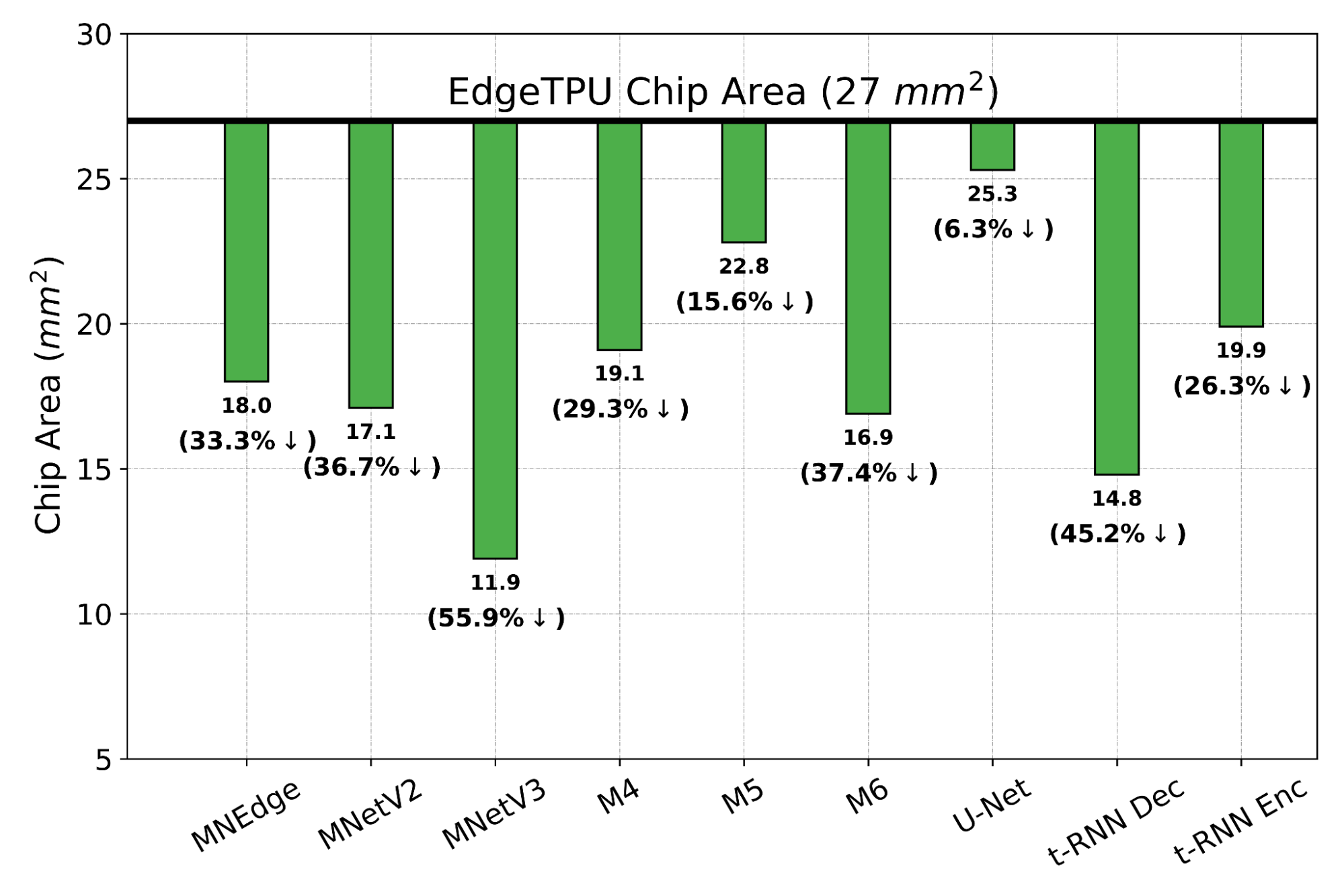
Does PRIME Outperform Custom-Engineered Accelerators? We evaluate PRIME on a variety of actual accelerator design tasks. We start by comparing the optimized accelerator design architected by PRIME targeted towards nine applications to the manually optimized EdgeTPU design. EdgeTPU accelerators are primarily optimized towards running applications in image classification, particularly MobileNetV2, MobileNetV3 and MobileNetEdge. Our goal is to check if PRIME can design an accelerator that attains a lower latency than a baseline EdgeTPU accelerator3, while also constraining the chip area to be under 27 mm2 (the default for the EdgeTPU accelerator). Shown below, we find that PRIME improves latency over EdgeTPU by 2.69x (up to 11.84x in t-RNN Enc), while also reducing the chip area usage by 1.50x (up to 2.28x in MobileNetV3), even though it was never trained to reduce chip area! Even on the MobileNet image-classification models, for which the custom-engineered EdgeTPU accelerator was optimized, PRIME improves latency by 1.85x.
Comparing latencies (lower is better) of accelerator designs suggested by PRIME and EdgeTPU for single-model specialization.
The chip area (lower is better) reduction compared to a baseline EdgeTPU design for single-model specialization.
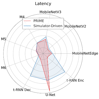
Designing Accelerators for New and Multiple Applications, Zero-Shot We now study how PRIME can use logged accelerator data to design accelerators for (1) multiple applications, where we optimize PRIME to design a single accelerator that works well across multiple applications simultaneously, and in a (2) zero-shot setting, where PRIME must generate an accelerator for new unseen application(s) without training on any data from such applications. In both settings, we train the contextual version of PRIME, conditioned on context vectors identifying the target applications and then optimize the learned model to obtain the final accelerator. We find that PRIME outperforms the best simulator-driven approach in both settings, even when very limited data is provided for training for a given application but many applications are available. Specifically in the zero-shot setting, PRIME outperforms the best simulator-driven method we compared to, attaining a reduction of 1.26x in latency. Further, the difference in performance increases as the number of training applications increases.
The average latency (lower is better) of test applications under zero-shot setting compared to a state-of-the-art simulator-driven approach. The text on top of each bar shows the set of training applications.
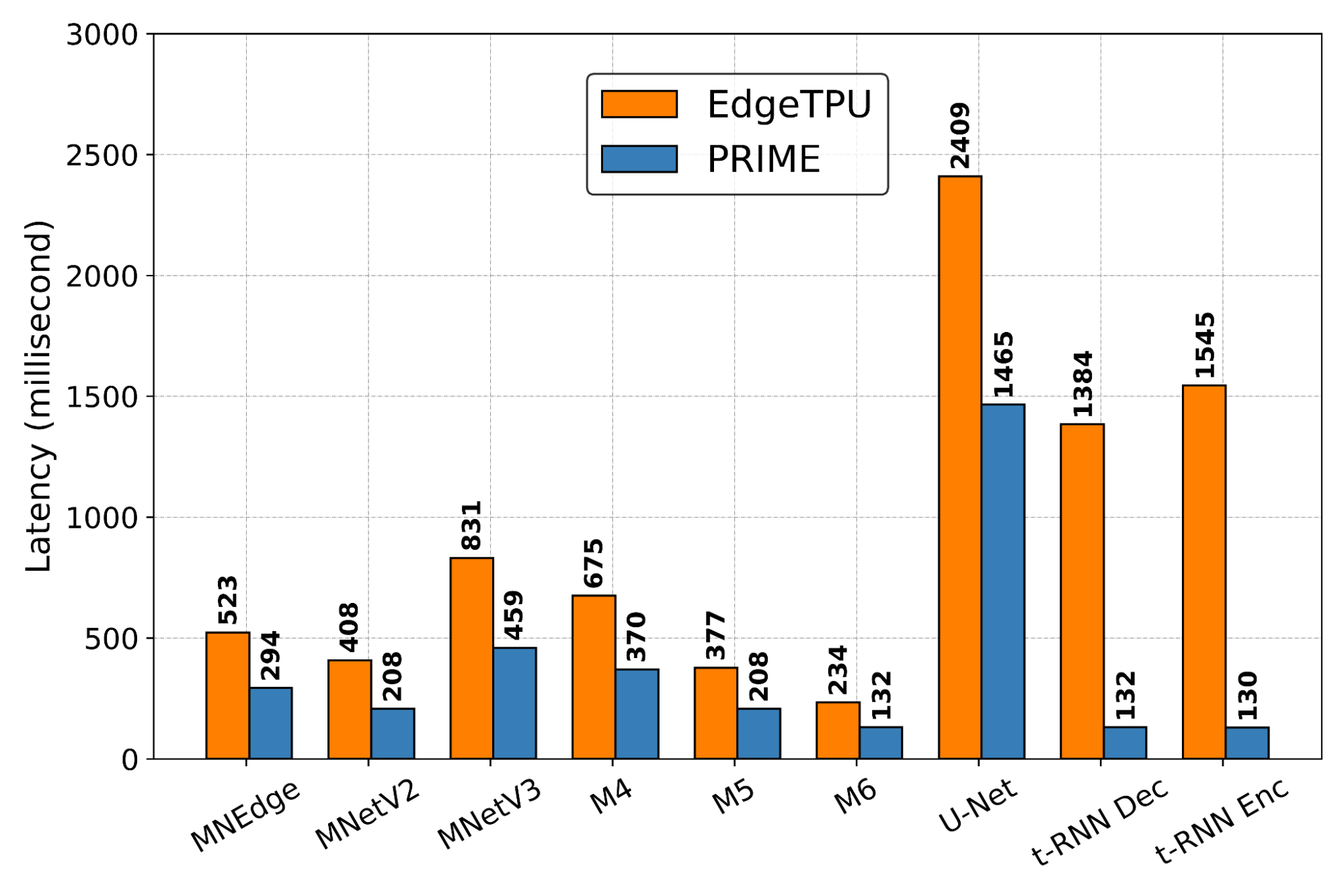
Closely Analyzing an Accelerator Designed by PRIME To provide more insight to hardware architecture, we examine the best accelerator designed by PRIME and compare it to the best accelerator found by the simulator-driven approach. We consider the setting where we need to jointly optimize the accelerator for all nine applications, MobileNetEdge, MobileNetV2, MobileNetV3, M4, M5, M64, t-RNN Dec, and t-RNN Enc, and U-Net, under a chip area constraint of 100 mm2. We find that PRIME improves latency by 1.35x over the simulator-driven approach.
Per application latency (lower is better) for the best accelerator design suggested by PRIME and state-of-the-art simulator-driven approach for a multi-task accelerator design. PRIME reduces the average latency across all nine applications by 1.35x over the simulator-driven method.
As shown above, while the latency of the accelerator designed by PRIME for MobileNetEdge, MobileNetV2, MobileNetV3, M4, t-RNN Dec, and t-RNN Enc are better, the accelerator found by the simulation-driven approach yields a lower latency in M5, M6, and U-Net. By closely inspecting the accelerator configurations, we find that PRIME trades compute (64 cores for PRIME vs. 128 cores for the simulator-driven approach) for larger Processing Element (PE) memory size (2,097,152 bytes vs. 1,048,576 bytes). These results show that PRIME favors PE memory size to accommodate the larger memory requirements in t-RNN Dec and t-RNN Enc, where large reductions in latency were possible. Under a fixed area budget, favoring larger on-chip memory comes at the expense of lower compute power in the accelerator. This reduction in the accelerator’s compute power leads to higher latency for the models with large numbers of compute operations, namely M5, M6, and U-Net.
Conclusion The efficacy of PRIME highlights the potential for utilizing the logged offline data in an accelerator design pipeline. A likely avenue for future work is to scale this approach across an array of applications, where we expect to see larger gains because simulator-driven approaches would need to solve a complex optimization problem, akin to searching for needle in a haystack, whereas PRIME can benefit from generalization of the surrogate model. On the other hand, we would also note that PRIME outperforms prior simulator-driven methods we utilize and this makes it a promising candidate to be used within a simulator-driven method. More generally, training a strong offline optimization algorithm on offline datasets of low-performing designs can be a highly effective ingredient in at the very least, kickstarting hardware design, versus throwing out prior data. Finally, given the generality of PRIME, we hope to use it for hardware-software co-design, which exhibits a large search space but plenty of opportunity for generalization. We have also released both the code for training PRIME and the dataset of accelerators.
Acknowledgments We thank our co-authors Sergey Levine, Kevin Swersky, and Milad Hashemi for their advice, thoughts and suggestions. We thank James Laudon, Cliff Young, Ravi Narayanaswami, Berkin Akin, Sheng-Chun Kao, Samira Khan, Suvinay Subramanian, Stella Aslibekyan, Christof Angermueller, and Olga Wichrowskafor for their help and support, and Sergey Levine for feedback on this blog post. In addition, we would like to extend our gratitude to the members of “Learn to Design Accelerators”, “EdgeTPU”, and the Vizier team for providing invaluable feedback and suggestions. We would also like to thank Tom Small for the animated figure used in this post.
1The infeasible accelerator designs stem from build errors in silicon or compilation/mapping failures. ↩ 2This is akin to adversarial examples in supervised learning – these examples are close to the data points observed in the training dataset, but are misclassified by the classifier. ↩ 3The performance metrics for the baseline EdgeTPU accelerator are extracted from an industry-based hardware simulator tuned to match the performance of the actual hardware. ↩ 4These are proprietary object-detection models, and we refer to them as M4 (indicating Model 4), M5, and M6 in the paper. ↩
Sign up now for DLI workshops at GTC and learn new technical skills from top experts across a range of fields including NLP, data science, deep learning, and more.
Are you looking to grow your technical skills with hands-on, instructor-led training? The NVIDIA Deep Learning Institute (DLI) is offering full-day workshops at NVIDIA GTC, March 21-24. Register for a workshop and learn how to create cutting-edge GPU-accelerated applications in AI, data science, or accelerated computing.
Each hands-on session gives you access to a fully configured GPU-accelerated server in the cloud, while you work with an instructor. Along with learning new skills, you will also earn an NVIDIA Deep Learning Institute certificate of subject matter competency, which can easily be added to your LinkedIn profile.
During GTC, all DLI workshops are offered at a special price of $149 (normally $500/seat.) NVIDIA Certified Instructors, who are technical experts in their fields, will be leading all eight DLI workshops.
Below are three subject matter experts looking forward to working with you next week.
Get to know some of DLI’s certified instructors
David Taubenheim, Senior Data Scientist at NVIDIA
David Taubenheim
David joined NVIDIA 3 years ago as a Senior Solutions Architect (SA) and plays a key role in a variety of strategic Data Science initiatives. He recently transitioned to the NVIDIA Inception Program teams, where he helps startup companies disrupt their market with accelerated computing and AI. He also completed a rotational assignment with the NVIDIA AI Applications team to develop better language models for neural machine translation. David’s technical specialty is NLP applications with GPU-accelerated SDKs.
“It happens pretty often that I’m approached by a client with a fantastic idea for a deep learning (DL) application but who isn’t quite sure how to get started. That’s one of the reasons I enjoy teaching the Fundamentals of Deep Learning course. I know I’m enabling people to do their best work and create something novel with DL. Each time we approach the end of a full day of hands-on labs, I can sense the ‘a-ha!’ moment as students learn how to use our SDKs and practice training DL models. When they enthusiastically want to take their finished code and final project home with them, I’m so pleased they’ll have a starting point for their idea!”
David earned a BS in Electrical Engineering from the University of Illinois Urbana-Champaign, and an MS from National Technological University. Before NVIDIA, he spent 25 years at Motorola and the Johns Hopkins Applied Physics Laboratory.
David Williams, FinTech Solutions Architect at NVIDIA
David Williams
As a Solutions Architect on the Financial Services team, David is helping payment companies adopt GPUs and AI. He teaches workshops focused on NLP applications, using models critical to understanding customer and market behavior. According to David, the wide-ranging use cases of NLP also provide an amazing opportunity to learn from students in completely distinct fields from the one he spends time with in his ‘day job.’
“I have a passion for teaching, which comes from both the joy of seeing others learn as well as the interaction with such a diverse range of students. DLI provides a great environment to lay the vital foundation in complex topics like deep learning and CUDA programming. I hope participants in my classes can easily grasp the most important concepts, no matter the level they came in at. Leading workshops at GTC, customer sites, and even internally at NVIDIA, introduces me to such varied backgrounds and experiences, my teaching provides me an opportunity to learn as well.”
David earned both a BS and MS in Computer Engineering from Northwestern University.
Along with being a Solutions Architect, Gunter manages many of the platform admin tasks for Europe, the Middle East, and Africa (EMEA) DLI workshops. While in that role he is actively spinning up GPU instances, minimizing downtime time for students and helping them get to work in their notebooks quickly.
Gunter Roth
“From my first day at NVIDIA, it was clear that teaching courses through DLI would be a simple, but highly efficient way to scale technical training for developers. Teaching the basics of CUDA or deep learning in rooms packed with eager students is certainly not always easy, but is a satisfying and rewarding experience. Using notebooks in the cloud helps students focus on the class, instead of spending time with CUDA drivers and SDK installation.”
He has a Master’s degree in geophysics from the Institut de Physique du Globe, in Paris and a PhD in seismology on the use of neural networks for interpreting geophysical data.
For a complete list of the 25 instructor-led workshops at GTC, visit the GTC Session Catalog. Several workshops are available in Taiwanese, Korean, and Japanese for attendees in their respective time zones.

 Use the high-level nvCOMP API for easy compression and decompression and the low-level API for more advanced workflows.
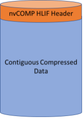


 Sign up now for DLI workshops at GTC and learn new technical skills from top experts across a range of fields including NLP, data science, deep learning, and more.

