I have been trying to find the cholesky decomposition of a bunch of randomly generated positive definite matrices but if the size of my matrix is any bigger than 2 by 2, tf gives me an error saying that the input is not correct for the tf.linalg.cholesky function.
I have even changed the data type to float64 but still no luck
This post defines NICs, SmartNICs, and lays out a cost-benefit analysis for NIC categories and use cases.
This post was originally published on the Mellanox blog.
Everyone is talking about data processing unit–based SmartNICs but without answering one simple question: What is a SmartNIC and what do they do?
NIC stands for network interface card. Practically speaking, a NIC is a PCIe card that plugs into a server or storage box to enable connectivity to an Ethernet network. A DPU-based SmartNIC goes beyond simple connectivity and implements network traffic processing on the NIC that would necessarily be performed by the CPU, in the case of a foundational NIC.
Some vendors’ definitions of a DPU-based SmartNIC are focused entirely on the implementation. This is problematic, as different vendors have different architectures. Thus, a DPU-based SmartNIC can be ASIC–, FPGA–, and system-on-a-chip-based. Naturally, vendors who make just one kind of NIC insist that only their type of NIC should qualify as a SmartNIC.
ASIC-based NIC
Excellent price performance
Vendor development cost high
Programmable and extensible
Flexibility is limited to predefined capabilities
FPGA-based NICs
Good performance but expensive
Difficult to program
Workload-specific optimization
SoC-based NICs + CPU
Good price performance
C programmable processors
Highest flexibility
Easiest programmability
There are various tradeoffs between these different implementations with regards to cost, ease of programming, and flexibility. An ASIC is cost-effective and may deliver the best price performance, but it suffers from limited flexibility. An ASIC-based NIC, like the NVIDIA ConnectX-5, can have a programmable data path that is relatively simple to configure. Ultimately, that functionality has limits based on what functions are defined within the ASIC. That can prevent certain workloads from being supported.
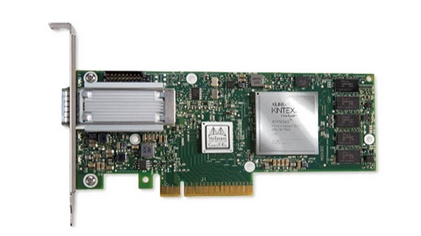
By contrast, an FPGA NIC, such as the NVIDIA Innova-2 Flex, is highly programmable. With enough time and effort, it can be made to support almost any functionality relatively efficiently, within the constraints of the available gates. However, FPGAs are notoriously difficult to program and expensive.
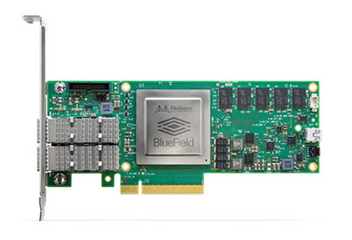
For more complex use cases, the SOC, such as the Mellanox BlueField DPU-programmable SmartNIC provides what appears to be the best DPU-based SmartNIC implementation option: good price performance, easy to program, and highly flexible.
Figure 1. SmartNIC implementation comparison
Focusing on how a particular vendor implements a DPU-based SmartNIC doesn’t address what it’s capable of or how it should be architected. NVIDIA actually has products based on each of these architectures that could be classified as DPU-based SmartNICs. In fact, customers use each of these products for different workloads, depending on their needs. So the focus on implementation—ASIC vs. FPGA vs. SoC—reverses the ‘form follows function’ philosophy that underlies the best architectural achievements.
Rather than focusing on implementation, I tweaked this PC Magazine encyclopedia entry to give a working definition of what makes a NIC a DPU-based SmartNIC:
DPU-based SmartNIC: A DPU-based network interface card (network adapter) that offloads processing tasks that the system CPU would normally handle. Using its own onboard processor, the DPU-based SmartNIC may be able to perform any combination of encryption/decryption, firewall, TCP/IP, and HTTP processing. SmartNICs are ideally suited for high-traffic web servers.
There are two things that I like about this definition. First, it focuses on the function more than the form. Second, it hints at this form with the statement, “…using its own onboard processor… to perform any combination of…” network processing tasks. So the embedded processor is key to achieving the flexibility to perform almost any networking function.
You could modernize that definition by adding that DPU-based SmartNICs might also perform network, storage, or GPU virtualization. Also, SmartNICs are also ideally suited for telco, security, machine learning, software-defined storage, and hyperconverged infrastructure servers, not just web servers.
NIC categories
Here’s how to differentiate three categories of NICs by the functions that the network adapters can support and use to accelerate different workloads:
Figure 2. Functional comparison of NIC categories
Here I’ve defined three categories of NICs, based on their ability to accelerate specific functionality:
Foundational NIC
Intelligent NIC (iNIC)
DPU-based SmartNIC
The foundational, or basic NIC simply moves network traffic and has few or no offloads, other than possibly SRIOV and basic TCP acceleration. It doesn’t save any CPU cycles and can’t offload packet steering or traffic flows. At NVIDIA, we don’t even sell a foundational NIC any more.
The NVIDIA ConnectX adapter family features a programmable data path and accelerates a range of functions that first became important in public cloud use cases. For this reason, I’ve defined this type of NIC as an iNIC, although today on-premises enterprise, telco, and private clouds are just as likely as public cloud providers to need this type of programmability and acceleration functionality. Another name for it could be smarterNIC without the capital “S.”
In many cases, customers tell us they need DPU based SmartNIC capabilities that are being offered by a competitor with either an FPGA or a NIC combined with custom, proprietary processing engines. But when customers really look at the functions they need for their specific workloads, ultimately they decide that the ConnectX family of iNICs provides all the function, performance, and flexibility of other so-called SmartNICs at a fraction of the power and cost. So by the definition of SmartNIC that some competitors use – our ConnectX NICs are indeed SmartNICs, though we might call them intelligent NICs or smarter NICs. Our FPGA NIC (Innova) is also a SmartNIC in the classic sense, and our SoC NIC (using BlueField) is the smartest of SmartNICs, to the extent that we could call them Genius NICs
So, what is a SmartNIC? A DPU-based SmartNIC is a network adapter that accelerates functionality and offloads it from the server (or storage) CPU.
How you should build a DPU-based SmartNIC and which SmartNIC is the best for each workload… well, the devil is in the details. It’s important to dig into exactly what data path and virtualization accelerations are available and how they can be used. If you’re interested, see my next post, Achieving a Cloud-Scale Architecture with DPUs.
For more information about SmartNIC use cases, see the following resources:
Learn how to simplify AI model deployment at the edge with NVIDIA Triton Inference Server on NVIDIA Jetson. Triton Inference Server is available on Jetson starting with the JetPack 4.6 release.
AI machine learning (ML) and deep learning (DL) are becoming effective tools for solving diverse computing problems in various fields including robotics, retail, healthcare, industrial, and so on. The need for low latency, real-time responsiveness, and privacy has moved running AI applications right at the edge.
However, deploying AI models in applications and services at the edge can be challenging for infrastructure and operations teams. Factors like diverse frameworks, end to end latency requirements, and lack of standardized implementations can make AI deployments challenging. In this post, we explore how to navigate these challenges and deploy AI models in production at the edge.
Here are the most common challenges of deploying models for inference:
Multiple model frameworks: Data scientists and researchers use different AI and deep learning frameworks like TensorFlow, PyTorch, TensorRT, ONNX Runtime, or just plain Python to build models. Each of these frameworks requires an execution backend to run the model in production. Managing multiple framework backends at the same time can be costly and lead to scalability and maintenance issues.
Different inference query types: Inference serving at the edge requires handling multiple simultaneous queries, queries of different types like real-time online predictions, streaming data, and a complex pipeline of multiple models. Each of these requires special processing for inference.
Constantly evolving models: With this ever-changing world, AI models are continuously retrained and updated based on new data and new algorithms. Models in production must be updated continuously without restarting the device. A typical AI application uses many different models. It compounds the scale of the problem to update the models in the field.
NVIDIA Triton Inference Server is an open-source inference serving software that simplifies inference serving by addressing these complexities. NVIDIA Triton provides a single standardized inference platform that can support running inference on multiframework models and in different deployment environments such as datacenter, cloud, embedded devices, and virtualized environments. It supports different types of inference queries through advanced batching and scheduling algorithms and supports live model updates. NVIDIA Triton is also designed to increase inference performance by maximizing hardware utilization through concurrent model execution and dynamic batching.
We brought Triton Inference Server to Jetson with NVIDIA JetPack 4.6, released in August 2021. With NVIDIA Triton, AI deployment can now be standardized across cloud, data center, and edge.
Key features
Here are some key features of NVIDIA Triton that help you simplify your model deployment in Jetson.
Figure 1. Triton Inference Server architecture on NVIDIA Jetson
Embedded application integration
Direct C-API integration is supported for communication between client applications and Triton Inference Server, though gRPC and HTTP/REST are supported. On Jetson, where both the client application and inference serving runs on the same device, client applications can call Triton Inference Server APIs directly with zero communication overhead. NVIDIA Triton is available as a shared library with a C API that enables the full functionality to be included directly in an application. This is best suited for Jetson-based, embedded applications.
Multiple framework support
NVIDIA Triton has natively integrated popular framework backends. Models developed in TensorFlow or ONNX or optimized with TRT can be run directly on Jetson without going through a conversion. NVIDIA Triton also supports flexibility to add custom backend. The developers get their choice and the infrastructure team streamlines the deployment with a single inference engine.
DLA support
Triton Inference Server on Jetson can run models on both GPU and DLA. DLA is the Deep Learning Accelerator available on Jetson Xavier NX and Jetson AGX Xavier.
Concurrent model execution
Triton Inference Server maximizes performance and reduces end-to-end latency by running multiple models concurrently on Jetson. These models can be all the same models, or different models from different frameworks. The GPU memory size is the only limitation to the number of models that can run concurrently.
Dynamic batching
Batching is a technique to improve inference throughput. There are two ways to batch inference requests: client and server batching. NVIDIA Triton implements server batching by combining individual inference requests together to improve inference throughput. It is dynamic because it builds a batch until a configurable latency threshold. When the threshold is met, NVIDIA Triton schedules the current batch for execution. The scheduling and batching decisions are transparent to the client requesting inference and is configured per model. Through dynamic batching, NVIDIA Triton maximizes throughput while meeting the strict latency requirements.
One of the examples of dynamic batching is where your application involves running both detection and classification models, where the input to classification model are the objects detected from the detection model. In this scenario, since there can be any number of detections to be classified, dynamic batching can make sure that the batch of detected objects can be created dynamically and classification can be run as a batched request, reducing the overall latency and improving the performance of your application.
Model ensembles
The model ensemble feature is used to create a pipeline of different models and pre– or post-processing operations to handle a variety of workloads. NVIDIA Triton ensembles represent a pipeline of one or more models and the connection of input and output tensors between those models. NVIDIA Triton can easily manage the execution of the entire pipeline just with a single inference request to an ensemble from the client application. As an example, applications trying to classify vehicles can use NVIDIA Triton model ensembles to run a vehicle detection model and then run vehicle classification model on the detected vehicles.
Custom backends
In addition to the popular AI backends, NVIDIA Triton also supports execution of custom C++ backends. These are useful to create special logic like pre– and post-processing or even regular models.
Dynamic model loading
NVIDIA Triton has a model control API that can be used to load and unload models dynamically. This enables the device to use the models when required by the application. Also, when a model gets retrained with new data it can be deployed by NVIDIA Triton for inference seamlessly without any application restarts or disruption to the service.
Conclusion
Triton Inference Server is released as a shared library for Jetson. NVIDIA Triton releases are made monthly, which adds new features and supports newest framework backends. For more information, see Triton Inference Server Support for Jetson and JetPack.
NVIDIA Triton helps with a standardized scalable production AI in every data center, cloud, and embedded device. It supports multiple frameworks, runs models on multiple computing engines like GPU and DLA, handles different types of inference queries. With the integration in NVIDIA JetPack, NVIDIA Triton can be used for embedded applications.
The NVIDIA Deep Learning Institute offers free courses for all experience levels in deep learning, accelerated computing, and accelerated data science.
For the first time, the NVIDIA Deep Learning Institute (DLI) is offering free, one-click notebooks for exploratory hands-on experience in deep learning, accelerated computing, and accelerated data science. The courses, ranging from as little as 10 minutes to 60 minutes, help expose you to the fundamental skills you need to do your life’s work.
Building a Brain in 10 Minutes
Learn how to build a brain in just 10 minutes! This free course teaches you how to build a simple neural network and explores the biological and psychological inspirations to the world’s first neural networks. You will explore how neural networks use data to learn and will get an understanding of the math behind a neuron.
Speed Up DataFrame Operations With RAPIDS cuDF
Get a glimpse into how to speed up dataframe operations with RAPIDS cuDF. This free notebook demonstrates significant speed-up by moving common DataFrame operations to the GPU with minimal changes to existing code. You will explore common data preparation processes and compare data manipulation performance using GPUs compared to CPUs.
An Even Easier Introduction to CUDA
Learn the basics of writing parallel CUDA kernels to run on NVIDIA GPUs. In this free course, you will launch massively parallel CUDA Kernels on an NVIDIA GPU, organize parallel thread execution for massive dataset sizes, manage memory between the CPU and GPU, and profile your CUDA code to observe performance gains.
More Options
Need more? Dive deeper and choose from an extensive catalog of hands-on, instructor-led workshops, or self-paced online training through DLI. You will have access to GPUs in the cloud and develop skills in AI, accelerated computing, accelerated data science, graphics and simulation, and more.
When you take a bold step forward, people notice. Today, the University of Florida advanced to No. 5 — in a three-way tie with University of California, Santa Barbara, and University of North Carolina, Chapel Hill — in U.S. News & World Report’s latest list of the best public colleges in the U.S. UF’s rise Read article >
An invisible AI-enabled keyboard created in South Korea accelerates one of the most ubiquitous tasks of our time: grinding through texts on mobile phones. The Invisible Mobile Keyboard, or IMK, created by researchers at the Korea Advanced Institute of Science and Technology, lets users blast through 51.6 words per minute while reporting lower strain levels. Read article >
TensorFlow Introduces the first version of ‘TensorFlow Similarity’. TensorFlow Similarity is an easy and fast Python package to train similarity models using TensorFlow.
One of the most essential features for an app or program to have in today’s world is a way to find related items. This could be similar-looking clothes, song titles that are playing on your computer/phone etc. More generally, it’s a vital part of many core information systems such as multimedia searches or recommenders because they rely on quickly retrieving related content/data – which would otherwise take up your time if not done efficiently.
Hi, anyone have working example of regression with text and numerical features? I’m struggling to get good result with multiple type of input like this
The early access version of the NVIDIA DOCA SDK was announced earlier this year at GTC. DOCA marks our focus on finding new ways to accelerate computing. The emergence of the DPU paradigm as the evolution of SmartNICs is finally here. We enable developers and application architects to squeeze more value out of general-purpose CPUs … Continued
The early access version of the NVIDIA DOCA SDK was announced earlier this year at GTC. DOCA marks our focus on finding new ways to accelerate computing. The emergence of the DPU paradigm as the evolution of SmartNICs is finally here. We enable developers and application architects to squeeze more value out of general-purpose CPUs by accelerating, offloading, and isolating the data center infrastructure to the DPU.
One of the most important ways to think about DOCA is as the DPU-enablement platform. DOCA enables the rapid consumption of DPU features into new and existing data center software stacks.
A modern data center consists of much more than simple network infrastructure. The key to operationally efficient and scalable data centers is software. Orchestration, provisioning, monitoring, and telemetry are all software components. Even the network infrastructure itself is mostly a function of software. The network OS used on the network nodes determines the feature set and drives many downstream decisions around operation tools and monitoring.
We call DOCA a software framework with an SDK, but it’s more than that. An SDK is a great place to start when thinking about what DOCA is and how to consume it. One frequent source of confusion is where components run. Which DOCA components are required on the host, and which are required on the DPU? Under which conditions would you need the SDK compared to the runtime environment? What are the DOCA libraries, exactly?
Overview
For those new to DOCA, this post demystifies some of the complexity around the DOCA stack and packaging. First, I’d like to revisit some terms and refine what they mean in the DOCA context.
SDK
This is a software development kit. In context, this is what an application developer would need to be able to write and compile software using DOCA. It contains runtimes, libraries, and drivers. Not everyone needs everything that is packaged with or is typically part of the SDK.
In a strict sense, an SDK is more about packaging software components, but it is also used to describe most concisely (though not entirely accurately) how the industry should think about what DOCA is and how to consume it. DOCA is primarily meant for use by application developers.
Runtime
This is the set of components required to run or execute a DOCA application. It contains the linked libraries and drivers that a DOCA application must have to run. In terms of packaging, it doesn’t need to contain the header files and sources to be able to write and build (compile) applications. DOCA applications can be written and built for either x86 or Arm, so there are different runtime bundles for each architecture.
Libraries
There are two different contexts here. In the broader and more general context, a library is a collection of resources used by applications. Library resources may include all sorts of data such as configuration, documentation, or help data; message templates; prewritten code; and subroutines, classes, values, or type specifications.
In the context of DOCA, libraries also provide a collection of more functional and useful behavior implementations. They provide well-defined interfaces by which that behavior is invoked.
For instance, the DOCA DPI library provides a framework for inspecting and acting on the contents of network packets.
To write a DPI application using the DPU RegEx accelerator from scratch would be a lot of work. You’d have to write all the preprocessing and postprocessing routines to parse packet headers and payload and then write a process to compile RegEx rules for the high-speed lookup on the accelerator.
Figure 1. The DOCA DPI library block.
Drivers
Device drivers provide an interface to a hardware device. This bit of software is the lowest level of abstraction. DOCA provides an additional layer of abstraction for the specific hardware functions of the DPU. This way, as the DPU hardware evolves, changes to the underlying hardware will not require DOCA applications to also update to follow new or different driver interfaces.
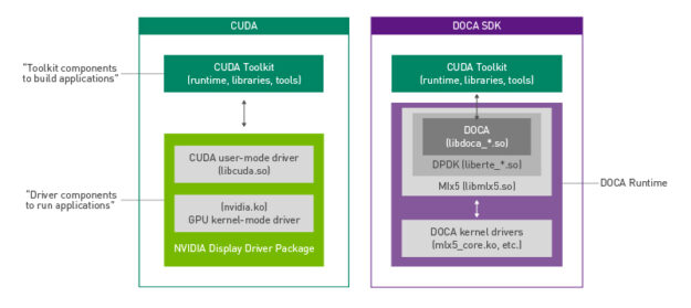
DOCA similarities to CUDA
Another useful way to think about DOCA packaging is through its similarities to CUDA. The DOCA runtime is meant to include all the drivers and libraries in a similar vein to what the NVIDIA display driver package provides for CUDA.
Applications that must invoke CUDA libraries for GPU processing only need the NVIDIA display driver package installed. Likewise, DOCA applications need only the runtime package for the specific architecture. In both cases, you have an additional set of packages and tools for integrating GPU or DPU functionality and acceleration into applications.
Figure 2. DOCA vs. the CUDA runtime and developer kit stack.
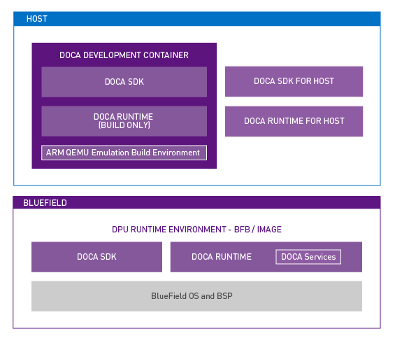
DOCA platform requirements
Another complicating factor can be sorting out which DOCA components are required on which platform. After all, the DPU runs its own OS, but also presents itself as a peripheral to the host OS.
DOCA applications can run on either the x86 host or on the DPU Arm cores. DOCA applications running on the x86 host are intended to use the DPU acceleration features through DOCA library calls. In terms of packaging, different OSs can mean different installation procedures for all these components, but luckily this isn’t as confusing as it seems for administrators.
For the NVIDIA BlueField DPU, all the runtime and SDK components are bundled with the OS image. It is possible to write, build, and compile DOCA applications on the DPU for rapid testing. All the DOCA components are there, but that isn’t always an ideal development environment. Having the SDK components built in and included with the DPU OS image makes it easier for everyone as it is the superset that contains the runtime components.
For the x86 host, there are many more individual components to consider. The packages that an administrator needs on the host depends, again, primarily on whether this host is a development environment or build server, and for which architecture. Or will the host run and execute applications that invoke DOCA libraries?
For x86 hosts destined to serve as a development environment, there is one additional consideration. For the development of DOCA applications that will run on x86 CPUs, an administrator needs the native x86 DOCA SDK for host packages. For developing Arm applications from an x86 host, NVIDIA has a prebuilt DOCA development container that manages all those cross-platform complexities.
In the simplest case for x86 hosts that only run or execute applications using DOCA, that’s what the DOCA Runtime for Host package would satisfy. It contains the minimum set of components to enable applications written using DOCA libraries to properly execute on the target machine. Figure 3 shows the different components across the two different OS domains.
Figure 3. DOCA Packaging between the host and the BlueField DPU.
Simplifying installation
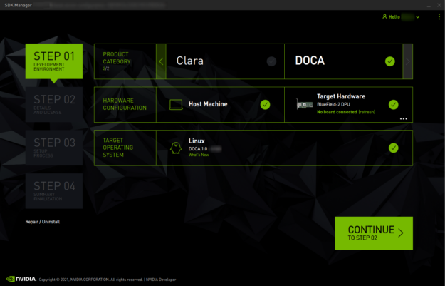
Now that I’ve explained how all that packaging works on the x86 host, I should mention that you have an easy way to get the right components installed in the right places. NVIDIA SDK Manager reduces the time and effort required to manage this packaging complexity. SDK Manager can not only install or repair the SDK components on the host but can also detect and install the OS onto the BlueField DPU, all through a graphical interface. Piece of cake!
Figure 4. SDK Manager graphical interface for setting up a DPU and installing DOCA components.
Summary
Hopefully, this post goes a long way in helping you understand and demystify DOCA and its packaging. To download DOCA software and get started, see the NVIDIA DOCA developer page.
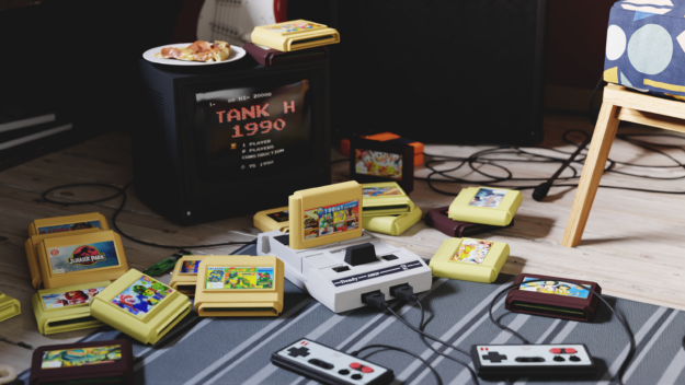
For this contest, we are asking creators to build and design their gaming space from the past—whether it’s a living room, bedroom, college dorm, or another area. The final submission can be big or small. Meaning you can create an entire room, or assemble a detailed close-up of a floor or desk from a space that inspired your passion for gaming or computer graphics.
Figure 1. Example of an acceptable close-up.
Figure 2. Example of an acceptable close-up.
Figure 3. Example of an acceptable full room view.
Creators must use Omniverse to design the 3D space in a retro style from the 80s, 90s, or 2000s. NVIDIA is collaborating with TurboSquid by Shutterstock, a leading 3D marketplace, to provide pre-made assets of consoles.
Participants can use any of the pre-selected assets from TurboSquid to build and design their space. Feel free to re-texture the assets, or even model the classic consoles or PCs from scratch.
Use any 3D software, workflow, or Connector to assemble the retro scene, creating the final render in Omniverse Create.
Entries will be judged on various criteria, including the use of Omniverse Create, the quality of the final render, and overall originality.
Deadline to submit the final render is October 26, 2021.
Contestants must provide one hero still image as their final entry, but can submit up to five images that highlight elements such as lighting variations or different angles, or specific assets within the scene.
The final entry needs to include a final high-res image, plus the final source files, including the USD file and the source file from the 3D application used.
The winners of the contest will be announced at our GTC conference in November.
Learn more about the Retroverse contest and start creating in Omniverse today. Share your submission on Twitter and Instagram by tagging @NVIDIAOmniverse with #CreateYourRetroverse.

 This post defines NICs, SmartNICs, and lays out a cost-benefit analysis for NIC categories and use cases.
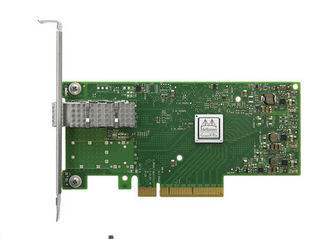


 Learn how to simplify AI model deployment at the edge with NVIDIA Triton Inference Server on NVIDIA Jetson. Triton Inference Server is available on Jetson starting with the JetPack 4.6 release.
 The early access version of the NVIDIA DOCA SDK was announced earlier this year at GTC. DOCA marks our focus on finding new ways to accelerate computing. The emergence of the DPU paradigm as the evolution of SmartNICs is finally here. We enable developers and application architects to squeeze more value out of general-purpose CPUs …
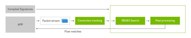
 Recreate the past with the new NVIDIA Omniverse retro design challenge.