This post discusses tensor methods, how they are used in NVIDIA, and how they are central to the next generation of AI algorithms. Tensors in modern machine learning Tensors, which generalize matrices to more than two dimensions, are everywhere in modern machine learning. From deep neural networks features to videos or fMRI data, the structure … Continued
This post discusses tensor methods, how they are used in NVIDIA, and how they are central to the next generation of AI algorithms.
Tensors in modern machine learning
Tensors, which generalize matrices to more than two dimensions, are everywhere in modern machine learning. From deep neural networks features to videos or fMRI data, the structure in these higher-order tensors is often crucial.
Deep neural networks typically map between higher-order tensors. In fact, it is the ability of deep convolutional neural networks to preserve and leverage local structure that made the current levels of performance possible, along with large datasets and efficient hardware. Tensor methods enable you to preserve and leverage that structure further, for individual layers or whole networks.
Figure 1. Deep Tensor Nets diagram.
Combining tensor methods and deep learning can lead to better models, including:
Better performance and generalization, through better inductive biases
Improved robustness, from implicit (low-rank structure) or explicit (tensor dropout) regularization
Parsimonious models, with a large reduction in the number of parameters
Computational speed-ups by operating directly and efficiently on factorized tensors
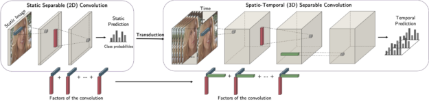
One example is factorized convolution. With a CP structure, it is possible to decompose the kernel of a convolution and express it efficiently as a separable one. This decouples the dimensions and enables you to transduct, such as training on 2D and generalizing to 3D while leveraging the information learned in 2D.
Figure 2. The process of factorized convolution: How 2D information turns into 3D information.
The proper implementation of tensor-based deep neural networks can be tricky. Major neural networks libraries such as PyTorch or TensorFlow do not provide layers based on tensor algebraic methods and have limited support for sparse tensors. In NVIDIA, we lead the development of a series of tools to make the use of tensor methods in deep learning seamless, through the TensorLy project and Minkowski Engine.
TensorLy ecosystem
TensorLy offers a high-level API for tensor methods, including decomposition and algebra.
It enables you to use tensor methods easily without requiring a lot of background knowledge. You can choose and seamlessly integrate with your computational backend of choice (NumPy, PyTorch, MXNet, TensorFlow, CuPy, or JAX), without having to change the code.
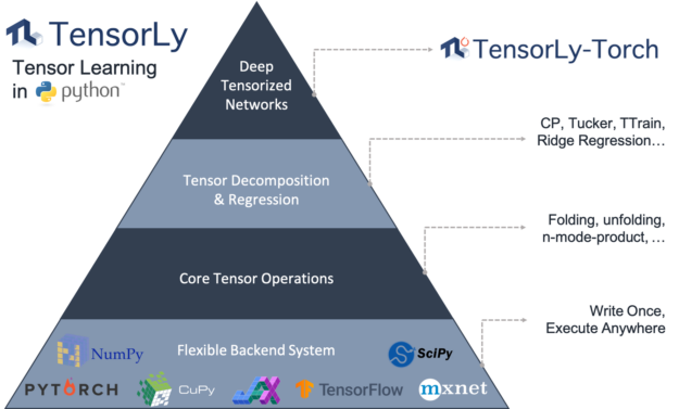
Figure 3. The TensorLy-Torch layer diagram.
TensorLy-Torch is a new library that builds on top of TensorLy and provides PyTorch layers implementing these tensor operations. They can be used out-of-the-box and readily integrated in any deep neural network. At the core of it is the concept of factorized tensors: tensors are represented, stored, and manipulated directly in decomposed form. Whenever possible, operations then directly operate on these decomposed tensors.
These factorized tensors can then be used to parametrize deep neural network layers efficiently, such as factorized convolutions and linear layers. Finally, tensor hooks enable you to apply techniques such as generalized lasso and tensor dropout seamlessly for improved generalization and robustness.
Spatially sparse tensors and Minkowski Engine
In many high-dimensional problems, data become sparse as the volume of the space increases faster. The sparsity is mostly embedded in the spatial dimension where you can compute distance. The most well-known example of such sparsity is 3D data, such as meshes and scans.
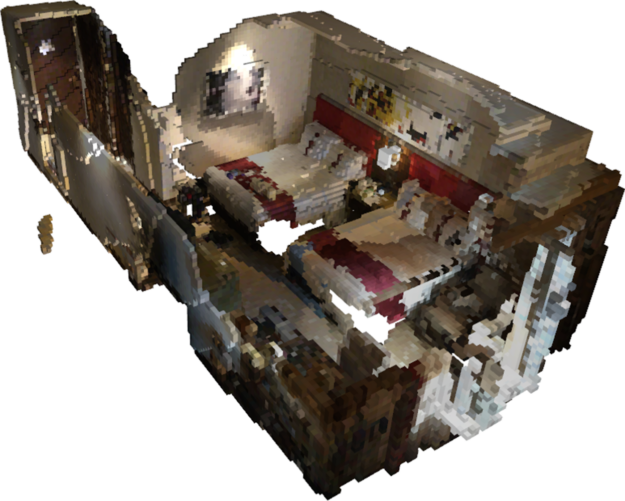
Figure 4. 3D Reconstruction of a Room with Two Beds.
Here’s an example 3D reconstruction of a room with two beds. The 3D bounding volume that it occupies can be quite large, but the data, or the 3D surface reconstruction, occupies only a fraction of the space. In this example, 95.5% of the space is empty and less than 5% contains a valid surface. Using a dense tensor to represent such data results in wasting not just large amounts of memory but also computation if you were to process such data.
For such cases, you could use a sparse representation that does not waste memory and computation on the empty space for building a neural network or a learning algorithm. Specifically, you use sparse tensors to represent such data, which is one of the most widely used representations for sparse data. Sparse tensors represent data using a pair of positions and values of nonzero values.
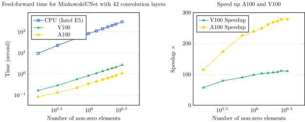
Minkowski Engine is a PyTorch extension that provides an extensive set of neural network layers for sparse tensors. All functions in Minkowski Engine support CPU and CUDA operations where CUDA operations accelerate over 100x over the top-of-the-line CPUs.
Figure 5. Sparse Representation Graphs: Number of non-zero elements over time, number of non-zero elements over speedup.
○ Quality assurance and audits are necessary for deep learning models. Current AI models require large data sets for training or a designed reward function that must be optimized. Algorithmically, AI is prone to optimizing behaviors that were not intended by the human designer. To help combat this, the AuditAI framework was developed to help audit these problems, which increases safety and ethical use of deep learning models during deployment.
When you purchased your last car, did you check for safety ratings or quality assurances from the manufacturer. Perhaps, like most consumers, you simply went for a test drive to see if the car offered all the features and functionality you were looking for, from comfortable seating to electronic controls.
Audits and quality assurance are the norm across many industries. Consider car manufacturing, where the production of the car is followed by rigorous tests of safety, comfort, networking, and so on, before deployment to end users. Based on this, we ask the question, “How can we design a similarly motivated auditing scheme for deep learning models?”
AI has enjoyed widespread success in real-world applications. Current AI models—deep neural networks in particular—do not require exact specifications of the type of desired behavior. Instead, they require large datasets for training, or a designed reward function that must be optimized over time.
While this form of implicit supervision provides flexibility, it often leads to the algorithm optimizing for behavior that was not intended by the human designer. In many cases, it also leads to catastrophic consequences and failures in safety-critical applications, such as autonomous driving and healthcare.
As these models are prone to failure, especially under domain shifts, it is important to know before their deployment when they might fail. As deep learning research becomes increasingly integrated with real world applications, we must come up with schemes of formally auditing deep learning models.
Semantically aligned unit tests
One of the biggest challenges in auditing is in understanding how we can obtain human-interpretable specifications that are directly useful to end users. We addressed this challenge through a sequence of semantically aligned unit tests. Each unit test verifies whether a predefined specification (for example, accuracy over 95%) is satisfied with respect to controlled and semantically aligned variations in the input space (for example, in face recognition, the angle relative to the camera).
We perform these unit tests by directly verifying the semantically aligned variations in an interpretable latent space of a generative model. Our framework, AuditAI, bridges the gap between interpretable formal verification of software systems and scalability of deep neural networks.
Figure 1. A general machine learning process for AI as it goes from a project to deployment.
Consider a typical machine learning production pipeline with three parties: the end user of the deployed model, verifier, and model designer. The verifier plays the critical role of verifying whether the model from the designer satisfies the need of the end user. For example, unit test 1 could be verifying whether a given face classification model maintains over 95% accuracy when the face angle is within d degrees. Unit test 2 could be checking under what lighting condition the model has over 86% accuracy. After verification, the end user can then use the verified specification to determine whether to use the trained DL model during deployment.
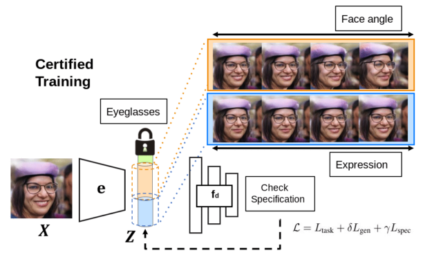
Figure 2. Deep networks undergo certified training to ensure that unit tests are likely to be satisfied.
Verified deployment
To verify the deep network for semantically aligned properties, we bridge it with a generative model, such that they share the same latent space and the same encoder that projects inputs to latent codes. In addition to verifying whether a unit test is satisfied, we can also perform certified training to ensure that the unit test is likely to be satisfied in the first place. The framework has appealing theoretical properties, and we show in our paper how the verifier is guaranteed to be able to generate a proof of whether the verification is true or false. For more information, see Auditing AI models for Verified Deployment under Semantic Specifications [LINK].
Verification and certified training of neural networks for pixel-based perturbations covers a much narrower range of semantic variations in the latent space, compared to AuditAI. To perform a quantitative comparison, for the same verified error, we project the pixel-bound to the latent space and compare it with the latent-space bound for AuditAI. We show that AuditAI can tolerate around 20% larger latent variations compared to pixel-based counterparts as measured by L2 norm, for the same verified error. For the implementation and experiments, we used NVIDIA V100 GPUs and Python with the PyTorch library.
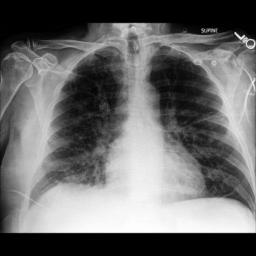
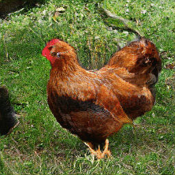
In Figure 3, we show qualitative results for generated outputs corresponding to controlled variations in the latent space. The top row shows visualizations for AuditAI, and the bottom row shows visualizations for pixel-perturbations for images of class hen on ImageNet, chest X-ray images with the condition pneumonia, and human faces with different degrees of smile respectively. From the visualizations, it is evident that wider latent variations correspond to a wider set of semantic variations in the generated outputs.
Figure 3. Top row: AuditAI visualizations, Bottom row: Visualizations for pixel-perturbations
Future work
In this paper, we developed a framework for auditing of deep learning (DL) models. There are increasingly growing concerns about innate biases in the DL models that are deployed in a wide range of settings and there have been multiple news articles about the necessity for auditing DL models before deployment. Our framework formalizes this audit problem, which we believe is a step towards increasing safety and the ethical use of DL models during deployment.
One of the limitations of AuditAI is that its interpretability is limited by that of the built-in generative model. While exciting progress has been made for generative models, we believe it is important to incorporate domain expertise to mitigate potential dataset biases and human error in both training and deployment.
Currently, AuditAI doesn’t directly integrate human domain experts in the auditing pipeline. It indirectly uses domain expertise in the curation of the dataset used for creating the generative model. Incorporating the former would be an important direction for future work.
Although we have demonstrated AuditAI primarily for auditing computer vision classification models, we hope that this would pave the way for more sophisticated domain-dependent AI-auditing tools and frameworks in language modeling and decision-making applications.
Acknowledgments
This work was conducted wholly at NVIDIA. We thank our co-authors De-An Huang, Chaowei Xiao, and Anima Anandkumar for helpful feedback, and everyone in the AI Algorithms team at NVIDIA for insightful discussions during the project.
Register now for the Sept. 21 instructor-led training from DLI covering training, accelerating, and optimizing a defect detection classifier.
NVIDIA GPUs are used to develop the most accurate automated inspection solutions for manufacturing semiconductors, electronics, automotive components, and assemblies. Along with accompanying software tools, GPUs enable efficient training of models for greater accuracy and optimized inference deployment at the edge. These models dramatically improve the accuracy of industrial inspection, resulting in reduced test escapes and increased yield at greater throughput.
The NVIDIA Deep Learning Institute (DLI) is offering an instructor-led class about training, accelerating, and optimizing a defect detection classifier.
You will start by exploring key challenges around industrial inspection, and problem formulation along with data curation, exploration, and formatting.
Then you will learn about the fundamentals of transfer learning, online augmentation, modeling, and fine-tuning.
By the end of the workshop, you’ll be familiar with the key concepts of optimized inference, performance assessment, and interpretation of deep learning models.
By participating in this workshop, you will learn how to:
Formulate an industrial inspection case study and curate datasets generated by automated optical inspection (AOI) machines.
Deal with the logistics and challenges of data handling in an industrial inspection workflow.
Extract meaningful insights from our dataset using pandas DataFrame and NumPy library.
Apply transfer learning to a deep learning classification model (Inception v3).
Fine-tune the deep learning model and set up evaluation metrics.
Optimize the trained Inception v3 model on an NVIDIA V100 Tensor Core GPU using NVIDIA TensorRT 5.
Experiment with FP16 half-precision fast inferencing with the V100’s Tensor Cores.
You will have access to a GPU-accelerated server in the cloud and earn an NVIDIA DLI certificate to demonstrate subject-matter competency and accelerate your career growth.
This workshop will be offered twice to accommodate both CEST and PDT timezones on: Tue, Sept. 21, 2021, 9 am–5 pm, CEST/EMEA, UTC+2 Tue, Sept. 21, 2021, 9 am–5 pm, PDT, UTC-7
Posted by Forrester Cole, Software Engineer and Tali Dekel, Research Scientist
Image and video editing operations often rely on accurate mattes — images that define a separation between foreground and background. While recent computer vision techniques can produce high-quality mattes for natural images and videos, allowing real-world applications such as generating synthetic depth-of-field, editing and synthesising images, or removing backgrounds from images, one fundamental piece is missing: the various scene effects that the subject may generate, like shadows, reflections, or smoke, are typically overlooked.
In “Omnimatte: Associating Objects and Their Effects in Video”, presented at CVPR 2021, we describe a new approach to matte generation that leverages layered neural rendering to separate a video into layers called omnimattes that include not only the subjects but also all of the effects related to them in the scene. Whereas a typical state-of-the-art segmentation model extracts masks for the subjects in a scene, for example, a person and a dog, the method proposed here can isolate and extract additional details associated with the subjects, such as shadows cast on the ground.
A state-of-the-art segmentation network (e.g., MaskRCNN) takes an input video (left) and produces plausible masks for people and animals (middle), but misses their associated effects. Our method produces mattes that include not only the subjects, but their shadows as well (right; individual channels for person and dog visualized as blue and green).
Also unlike segmentation masks, omnimattes can capture partially-transparent, soft effects such as reflections, splashes, or tire smoke. Like conventional mattes, omnimattes are RGBA images that can be manipulated using widely-available image or video editing tools, and can be used wherever conventional mattes are used, for example, to insert text into a video underneath a smoke trail.
Layered Decomposition of Video To generate omnimattes, we split the input video into a set of layers: one for each moving subject, and one additional layer for stationary background objects. In the example below, there is one layer for the person, one for the dog, and one for the background. When merged together using conventional alpha blending, these layers reproduce the input video.
Besides reproducing the video, the decomposition must capture the correct effects in each layer. For example, if the person’s shadow appears in the dog’s layer, the merged layers would still reproduce the input video, but inserting an additional element between the person and dog would produce an obvious error. The challenge is to find a decomposition where each subject’s layer captures only that subject’s effects, producing a true omnimatte.
Our solution is to apply our previously developed layered neural rendering approach to train a convolutional neural network (CNN) to map the subject’s segmentation mask and a background noise image into an omnimatte. Due to their structure, CNNs are naturally inclined to learn correlations between image effects, and the stronger the correlation between the effects, the easier for the CNN to learn. In the above video, for example, the spatial relationships between the person and their shadow, and the dog and its shadow, remain similar as they walk from right to left. The relationships change more (hence, the correlations are weaker) between the person and the dog’s shadow, or the dog and the person’s shadow. The CNN learns the stronger correlations first, leading to the correct decomposition.
The omnimatte system is shown in detail below. In a preprocess, the user chooses the subjects and specifies a layer for each. A segmentation mask for each subject is extracted using an off-the-shelf segmentation network, such as MaskRCNN, and camera transformations relative to the background are found using standard camera stabilization tools. A random noise image is defined in the background reference frame and sampled using the camera transformations to produce per-frame noise images. The noise images provide image features that are random but consistently track the background over time, providing a natural input for the CNN to learn to reconstruct the background colors.
The rendering CNN takes as input the segmentation mask and the per-frame noise images and produces the RGB color images and alpha maps, which capture the transparency of each layer. These outputs are merged using conventional alpha-blending to produce the output frame. The CNN is trained from scratch to reconstruct the input frames by finding and associating the effects not captured in a mask (e.g., shadows, reflections or smoke) with the given foreground layer, and to ensure the subject’s alpha roughly includes the segmentation mask. To make sure the foreground layers only capture the foreground elements and none of the stationary background, a sparsity loss is also applied on the foreground alpha.
A new rendering network is trained for each video. Because the network is only required to reconstruct the single input video, it is able to capture fine structures and fast motion in addition to separating the effects of each subject, as seen below. In the walking example, the omnimatte includes the shadow cast on the slats of the park bench. In the tennis example, the thin shadow and even the tennis ball are captured. In the soccer example, the shadow of the player and the ball are decomposed into their proper layers (with a slight error when the player’s foot is occluded by the ball).
This basic model already works well, but one can improve the results by augmenting the input of the CNN with additional buffers such as optical flow or texture coordinates.
Applications Once the omnimattes are generated, how can they be used? As shown above, we can remove objects, simply by removing their layer from the composition. We can also duplicate objects, by repeating their layer in the composition. In the example below, the video has been “unwrapped” into a panorama, and the horse duplicated several times to produce a stroboscopic photograph effect. Note that the shadow that the horse casts on the ground and onto the obstacle is correctly captured.
A more subtle, but powerful application is to retime the subjects. Manipulation of time is widely used in film, but usually requires separate shots for each subject and a controlled filming environment. A decomposition into omnimattes makes retiming effects possible for everyday videos using only post-processing, simply by independently changing the playback rate of each layer. Since the omnimattes are standard RGBA images, this retiming edit can be done using conventional video editing software.
The video below is decomposed into three layers, one for each child. The children’s initial, unsynchronized jumps are aligned by simply adjusting the playback rate of their layers, producing realistic retiming for the splashes and reflections in the water.
In the original video (left), each child jumps at a different time. After editing (right), everyone jumps together.
It’s important to consider that any novel technique for manipulating images should be developed and applied responsibly, as it could be misused to produce fake or misleading information. Our technique was developed in accordance with our AI Principles and only allows rearrangement of content already present in the video, but even simple rearrangement can significantly alter the effect of a video, as shown in these examples. Researchers should be aware of these risks.
Future Work There are a number of exciting directions to improve the quality of the omnimattes. On a practical level, this system currently only supports backgrounds that can be modeled as panoramas, where the position of the camera is fixed. When the camera position moves, the panorama model cannot accurately capture the entire background, and some background elements may clutter the foreground layers (sometimes visible in the above figures). Handling fully general camera motion, such as walking through a room or down a street, would require a 3D background model. Reconstruction of 3D scenes in the presence of moving objects and effects is still a difficult research challenge, but one that has seen promising recent progress.
On a theoretical level, the ability of CNNs to learn correlations is powerful, but still somewhat mysterious, and does not always lead to the expected layer decomposition. While our system allows for manual editing when the automatic result is imperfect, a better solution would be to fully understand the capabilities and limitations of CNNs to learn image correlations. Such an understanding could lead to improved denoising, inpainting, and many other video editing applications besides layer decomposition.
Acknowledgements Erika Lu, from the University of Oxford, developed the omnimatte system during two internships at Google, in collaboration with Google researchers Forrester Cole, Tali Dekel, Michael Rubinstein, William T. Freeman and David Salesin, and University of Oxford researchers Weidi Xie and Andrew Zisserman.
Thank you to the friends and families of the authors who agreed to appear in the example videos. The “horse jump low”, “lucia”, and “tennis” videos are from the DAVIS 2016 dataset. The soccer video is used by permission from Online Soccer Skills. The car drift video was licensed from Shutterstock.
Unreal Engine developers receive access to several NVIDIA updates. Our custom branch of Unreal Engine 4.27 (NvRTX) improves Deep Learning Super Sampling (DLSS), RTX Global Illumination (RTXGI), RTX Direct Illumination (RTXDI), and NVIDIA Real-Time Denoisers (NRD).
Custom RTX Branch of UE4.27 Drops, Global Illumination and Low Latency Solutions Level Up
Today, Unreal Engine developers receive access to several NVIDIA updates. Our custom branch of Unreal Engine 4.27 (NvRTX) improves Deep Learning Super Sampling (DLSS), RTX Global Illumination (RTXGI), RTX Direct Illumination (RTXDI), and NVIDIA Real-Time Denoisers (NRD). The Unreal Engine RTXGI plugin has been updated, making it easy to add the latest version of this global illumination SDK (1.1.40) to your game. And NVIDIA Reflex is now a standard feature in Unreal Engine 4.27. Details for each product are below.
NVIDIA has made it easy for game developers to add leading-edge technologies to their Unreal Engine (UE4) games by providing custom UE4 branches for NVIDIA technologies on GitHub. NvRTX 4.27 will shorten your development cycles and help make your games look even more stunning.
In NvRTX 4.27, RTX Direct Illumination (RTXDI) and NVIDIA Real-Time Denoisers (NRD) improved support for Metahuman hair. Deep Learning Super Sampling (DLSS) added softening capability to the sharpness slider, and provided a workaround for packaged builds not initializing DLSS on d3d11 devices. RTXGI increased the number of volumes supported in the indirect lighting pass from 6 to 12, made screen-space indirect lighting resolution adjustable through cvars, and supported blending of more than 2 volumes.
Leveraging the power of ray tracing, RTXGI provides scalable solutions to compute multi-bounce indirect lighting without bake times, light leaks, or expensive per-frame costs. RTXGI is supported on any DXR-enabled GPU, and is an ideal starting point to bring the benefits of ray tracing to your existing tools, knowledge, and capabilities.
As in the NvRTX update, this plugin update doubles the number of volumes supported in the indirect lighting pass, enables developers to adjust screen-space indirect lighting resolution, and supports the blending of more than 2 volumes.
Reflex (now available in Unreal Engine 4.27)
The NVIDIA Reflex SDK allows game developers to implement a low latency mode that aligns game engine work to complete just-in-time for rendering, eliminating the GPU render queue and reducing CPU back pressure in GPU-bound scenarios. As a developer, System Latency (click-to-display) can be one of the hardest metrics to optimize for. In addition to latency reduction functions, the SDK also features measurement markers to calculate both Game and Render Latency – great for debugging and in-game performance counters.
NVIDIA Reflex is now mainlined within UE4.27 and natively supported. To get started adding NVIDIA Reflex to your game, check out our easy step by step integration guide.
Read about how deep learning models are used for an automated pick and place system, a feature more and more advanced warehouses are implementing.
Advanced warehouses process up to hundreds-of-thousands of orders a day. Fulfilling these quantities requires a lot of inventory, physical space, and complex workflows to support the high volume of items picked.
In addition, micro-fulfillment centers are becoming increasingly popular to fill same-day delivery orders from customers.
Operating these types of advanced facilities and machinery—along with a high volume of resources efficiently— requires skilled workers. While this workforce is shrinking, investing in edge computing and AI can help.
Shrinking Workforce
Modern warehouses feature robust automation. Autonomous machines and vehicles move products around warehouses, conveyor systems move goods into shipping containers, and use advanced 3D grids to provide pick-and-sort systems that pack products intelligently. But even with the current level of automation, modern warehouses are still labor intensive.
If boxes are different sizes, automated packing is difficult and often done manually. Some items are large and heavy, requiring a forklift and a driver to move. Finding and retaining employees is a challenge and COVID-19 protocols have exacerbated the problem. And while the workforce is shrinking, the warehouse industry is growing rapidly. The next generation of warehouses needs to focus on automation to succeed.
Deep Learning for Advanced Industry
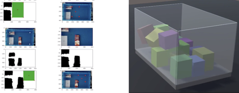
Advancements in deep learning and edge computing provide intelligence and automate more processes of warehouses. Automated pick and place systems are an example of an operation advanced warehouses are implementing. In a pick and place system, an autonomous machine identifies an object among other objects in a bin, then selects, and places that object for packing elsewhere.
For this system to be automated, many different deep learning models are required. That’s because some objects are very hard to detect with computer vision, like translucent, reflective, or non-uniform objects.
The walkthrough below outlines how deep learning models are used for an automated pick and place system.
First, the object grasp point needs to be identified. This is the simplest deep learning model, but an important function for automation. Once it is known where to grasp an object, it is necessary to understand how the object exists in 3D space. Therefore, a depth estimation model is needed that allows the pick and place system to understand the depth of the object in the environment.
Transparent or reflective objects have a higher error rate for detection.
Once the object has been picked, it needs to be placed. To do this, an orientation model is used to determine the position in space of the item picked.
An orientation model helps us understand how an object needs to be placed or packed.
Combining those models and others allows for effective bin packing.
Multilayer bin packing is tested through simulation models.
Pick and place systems showcase just some examples of models being used by retailers to improve warehouse automation.
When using RAPIDS, practitioners can quickly accelerate data science workloads on NVIDIA GPUs, and with Saturn Cloud allows practitioners and enterprises to focus on solving their business challenges.
GPU-accelerated computing is a game-changer for data practitioners and enterprises, but leveraging GPUs can be challenging for data professionals. RAPIDS remediates these challenges by abstracting the complexities of accelerated data science through familiar interfaces. When using RAPIDS, practitioners can quickly accelerate data science workloads on NVIDIA GPUs, reducing operations like data loading, processing, and training from hours to seconds.
Managing large-scale data science infrastructure presents significant challenges. With Saturn Cloud, managing GPU-based infrastructure is made easier, allowing practitioners and enterprises to focus on solving their business challenges.
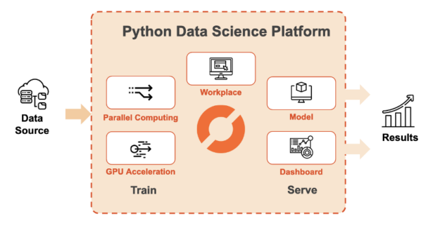
What is Saturn Cloud?
Saturn Cloud is an end-to-end platform that makes Python-based data science accessible with scalable computing resources in the cloud. Saturn Cloud offers an easy path to moving to the cloud with no cost, setup, or infrastructure work. This includes access to GPU-equipped computing resources with pre-built environments that include tools like RAPIDS, PyTorch, and TensorFlow.
Users are able to write their code in a hosted JupyterLab environment or connect their own IDE (integrated development environment) using SSH. As their data sizes increase, users can scale up to a GPU-enabled Dask cluster to execute code across a distributed network of machines. After a data pipeline, model, or dashboard is developed, users can deploy it to a persistent location or create a job to run it on a schedule.
Figure 1: Saturn Cloud provides a Python-based platform for large-scale data science.
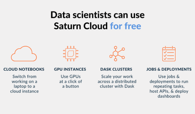
In addition to Saturn Cloud’s enterprise offering, Saturn Cloud also provides hosted offerings where anyone can get started with GPU-accelerated data science for free. The Hosted Free plan includes 10 hours of a Jupyter workspace and 3 hours of a Dask cluster per month. If you want more resources, you can upgrade to the Hosted Pro plan and pay as you go.
Figure 2: Users have access to notebooks, GPUs, clusters, and scheduling tools on Saturn Cloud Hosted.
Saturn Cloud provides an easy-to-use platform for GPU-accelerated data science applications. With this platform, GPUs become a core component of the everyday data science stack.
Get started with RAPIDS on Saturn Cloud
You can quickly get going with RAPIDS after creating a free account on Saturn Cloud Hosted. In this section, we show how Saturn Cloud can be used to train a machine learning model on New York taxi data using RAPIDS. We then go further and run RAPIDS on a Dask cluster. By combining RAPIDS and Dask, you can use a network of multi-node GPU systems to train a model far faster than with a single GPU.
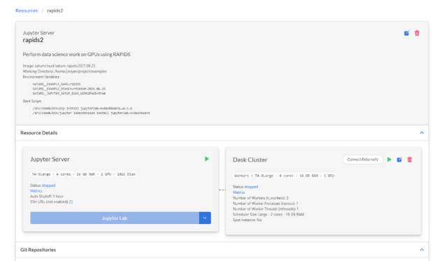
After creating your free account on Saturn Cloud Hosted, open the service and go to the “Resources” page. From there, look at the premade resource templates and click the one labeled RAPIDS.
Figure 3: Saturn Cloud has pre-configured RAPIDS images to ease getting started with GPUs.
You will be taken to the newly created resource. Everything is already set up for you here to run your code on GPU hardware, with a Docker image that has all the necessary Python and RAPIDS packages installed.
Figure 4: Saturn Cloud sets up a RAPIDS-equipped Jupyter server and Dask cluster.
Common PyData packages such as NumPy, SciPy, pandas, and scikit-learn
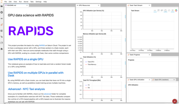
Click the play button on the “Jupyter Server” and “Dask Cluster” cards to start your resources. Now your cluster is ready to go; follow along to see how a GPU can significantly speed up model training time.
Figure 5: Pre-built RAPIDS environment with single and multi-GPU backends.
Train a random forest model with RAPIDS
For this exercise, we will use the NYC Taxi dataset. We will load a CSV file, select our features, then train a random forest model. To illustrate the runtime speedups we can achieve using RAPIDS on a GPU, we’ll first use traditional CPU-based PyData packages like pandas and scikit-learn.
Our machine learning model answers the question:
> Based on characteristics that can be known at the beginning of a trip, will this trip result in a high tip?
The dependent variable here is the “tip percentage”, or the dollar amount of the tip divided by the dollar amount of the ride cost. We’ll use pickup destination, drop-off destination, and the number of passengers as independent variables.
To follow along, you can copy the code chunks below into a new notebook in the Saturn Cloud JupyterLab interface. Alternatively, you can download the entire notebook here. First, we’ll set up a context manager to time different portions of the code:
 from time import time
 from contextlib import contextmanager

 times = {}

 @contextmanager
 def timing(description: str) -> None:
        start = time()
        yield
        elapsed = time() - start
        times[description] = elapsed
        print(f"{description}: {round(elapsed)} seconds")
Then we will pull a CSV file down from the NYC Taxi S3 bucket. Note that we could read the file directly from S3 into a dataframe. However, we want to separate network IO time from processing time on the CPU or GPU, and in case we want to run this step with modifications dozens of times, we won’t have to incur the network cost multiple times.
Before we get to the GPU part, let’s see how this would look with traditional PyData packages such as pandas and scikit-learn that use the CPU for computations.
 import pandas as pd
 from sklearn.ensemble import RandomForestClassifier as RFCPU

 with timing("CPU: CSV Load"):
        taxi_cpu = pd.read_csv(
        "data.csv",
        parse_dates=["tpep_pickup_datetime", "tpep_dropoff_datetime"],
        )

 X_cpu = (
        taxi_cpu[["PULocationID", "DOLocationID", "passenger_count"]]
        .fillna(-1)
 )
 y_cpu = (taxi_cpu["tip_amount"] > 1)

 rf_cpu = RFCPU(n_estimators=100, n_jobs=-1)

 with timing("CPU: Random Forest"):
        _ = rf_cpu.fit(X_cpu, y_cpu)
The CPU code will take a few minutes, so go ahead and open a new notebook for the GPU code. You’ll notice that the GPU code looks almost identical to the CPU code, except we’re swapping out `pandas` for `cudf` and `scikit-learn` for `cuml`. The RAPIDS packages resemble typical PyData packages on purpose, making it as easy as possible to enable your code to run on GPUs!
 import cudf
 from cuml.ensemble import RandomForestClassifier as RFGPU

 with timing("GPU: CSV Load"):
        taxi_gpu = cudf.read_csv(
        "data.csv",
        parse_dates=["tpep_pickup_datetime", "tpep_dropoff_datetime"],
        )

 X_gpu = (
        taxi_gpu[["PULocationID", "DOLocationID", "passenger_count"]]
        .astype("float32")
        .fillna(-1)
 )
 y_gpu = (taxi_gpu["tip_amount"] > 1).astype("int32")

 rf_gpu = RFGPU(n_estimators=100)

 with timing("GPU: Random Forest"):
        _ = rf_gpu.fit(X_gpu, y_gpu)
You should have been able to copy this into a new notebook and execute the whole thing before the CPU version finished. Once that’s done, check out the difference in the runtimes of each.
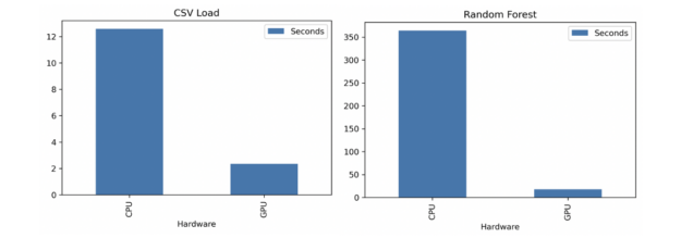
With the CPU, CSV loading took 13 seconds while random forest training took 364 seconds (6 minutes). With the GPU, CSV loading took 2 seconds while random forest training took 18 seconds. That’s 7x faster CSV loading and 20x faster random forest training.
Figure 6: RAPIDS + Saturn Cloud help users solve their challenges instead of waiting on processes.
Using RAPIDS + Dask for your big data problems
While a single GPU is powerful enough for many use cases, modern data science use cases often benefit from increasingly large datasets to generate more accurate and profound insights. Many use cases require scale-out infrastructure consisting of multiple GPUs or nodes to churn through workloads. RAPIDS pairs well with Dask to support scaling out to large GPU clusters.
With Saturn Cloud, you can connect to a GPU-powered Dask cluster from the same project we were using earlier. Then, to utilize Dask on GPUs, you would swap out the cudf package for dask_cudf for loading data, and use the cuml.dask submodule for machine learning. Notice now that we’re using glob syntax with dask_cudf.read_csv to load in data for all of 2019, rather than a single month as we did previously. This processes approximately 12x the amount of data as our previous example but only takes 90 seconds with the GPU cluster.
Make Accelerated Data Science Easy with RAPIDS and Saturn Cloud
This example showed how easy it is to accelerate your data science workloads with RAPIDS on a GPU or a GPU Dask cluster. Using RAPIDS can increase training times by an order of magnitude, which can help you iterate your models more quickly. With Saturn Cloud, you can spin up Jupyter Notebooks, Dask clusters, and other cloud resources right when you want them.
To get started with GPUs on Saturn Cloud, create a free account here and see what the power of accelerated compute can bring to your data science workloads.
Promising more accurate predictions in an era of rapid climate change, a new tool is harnessing deep learning to help better forecast Arctic sea ice conditions months into the future. As described in a paper published in the science journal Nature Communications Thursday, the new AI tool, dubbed IceNet, could lead to improved early-warning systems Read article >
AI has transformed synthesized speech from the monotone of robocalls and decades-old GPS navigation systems to the polished tone of virtual assistants in smartphones and smart speakers. But there’s still a gap between AI-synthesized speech and the human speech we hear in daily conversation and in the media. That’s because people speak with complex rhythm, Read article >
I have implemented a simple helper module to code layers easier. It has embedding layers, layer normalization, multi-head attention and an Adam optimizer implemented from ground up. I may have made mistakes and not followed JAX best practices since I’m new to JAX. Let me know if you see any opportunities for improvement.

 This post discusses tensor methods, how they are used in NVIDIA, and how they are central to the next generation of AI algorithms. Tensors in modern machine learning Tensors, which generalize matrices to more than two dimensions, are everywhere in modern machine learning. From deep neural networks features to videos or fMRI data, the structure … Continued
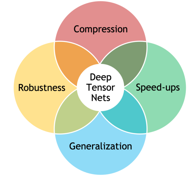
 ○ Quality assurance and audits are necessary for deep learning models. Current AI models require large data sets for training or a designed reward function that must be optimized. Algorithmically, AI is prone to optimizing behaviors that were not intended by the human designer. To help combat this, the AuditAI framework was developed to help audit these problems, which increases safety and ethical use of deep learning models during deployment.
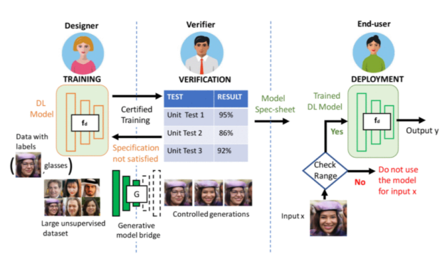

 Register now for the Sept. 21 instructor-led training from DLI covering training, accelerating, and optimizing a defect detection classifier.
  5.
5.


 Unreal Engine developers receive access to several NVIDIA updates. Our custom branch of Unreal Engine 4.27 (NvRTX) improves Deep Learning Super Sampling (DLSS), RTX Global Illumination (RTXGI), RTX Direct Illumination (RTXDI), and NVIDIA Real-Time Denoisers (NRD).
 Read about how deep learning models are used for an automated pick and place system, a feature more and more advanced warehouses are implementing.
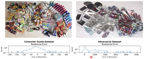
 When using RAPIDS, practitioners can quickly accelerate data science workloads on NVIDIA GPUs, and with Saturn Cloud allows practitioners and enterprises to focus on solving their business challenges.