Learn how to up a confidential AI inference service. Using TensorFlow Serving, we’ll showcase a multi-stakeholder scenario including cloud service provider, model owner, inference service provider, and users.
What would be a good way to continuously add user ratings to the model, instead of training it from scratch with the complete dataset every time there is an update? What I would like to avoid is having to fetch and process the complete dataset every time there are only a few new user ratings. Is this even possible?
Or, in other words: What are options for doing this in real time? Re-training the model from scratch every time a user rates something seems a bit of an overkill for whatever server that processes this data.
I would be very thankful for some insights and/or somebody pointing me in the right direction with this. Thanks!
I am trying to learn Tensorflow, but most of the courses and tutorials focus on the v1.Session style code. Specifically I am looking at the estimators. When consulting the Tensorflow documentation there is a big red notice:
Warning: Estimators are not recommended for new code. Estimators run
-style code which is more difficult to write correctly, and can behave unexpectedly, especially when combined with TF 2 code. Estimators do fall under compatibility guarantees, but will receive no fixes other than security vulnerabilities. See the migration guide for details.
Looking at the migration guide, they only mention estimators in the capacity that they are still compatible.
My question
What are we to use in place of the estimators?
A secondary question, where can I get some good training material on purely v2.5 stuff that outlines a “clean” way to code networks without Session or anything that is going to be imminently deprecated?
Solving a mystery that stumped scientists for decades, last November a group of computational biologists from Alphabet’s DeepMind used AI to predict a protein’s structure from its amino acid sequence. Not even a year later, a new study offers a more powerful model, capable of computing protein structures in as little as 10 minutes, on … Continued
Solving a mystery that stumped scientists for decades, last November a group of computational biologists from Alphabet’s DeepMind used AI to predict a protein’s structure from its amino acid sequence.
Not even a year later, a new study offers a more powerful model, capable of computing protein structures in as little as 10 minutes, on one gaming computer.
The research, from scientists at the University of Washington (UW), holds promise for faster drug development, which could unlock solutions for treating diseases like cancer.
Present in every cell in the body, proteins play a role in many processes such as blood clotting, hormone regulation, immune system response, vision, and cell and tissue repair. Made from long chains of amino acids that interact to form a folded three-dimensional structure, the shape of a protein determines its function.
Unfolded or misfolded proteins are also thought to cause degenerative disorders including cystic fibrosis, Alzheimer’s disease, Parkinson’s disease, and Huntington’s disease. Understanding and predicting how a protein structure develops could help scientists design effective interventions for many of these diseases.
The researchers at UW developed the RoseTTAFold model by creating a three-track neural network that simultaneously considers the sequence patterns, amino acid interaction, and possible three-dimensional structure of a protein.
To train the model, the team used discontinuous crops of protein segments, with 260 unique amino acid elements. With the cuDNN-accelerated PyTorch deep learning framework, and NVIDIA GeForce 2080 GPUs, this information flows back and forth within the deep learning model. The network is then able to deduce a protein’s chemical parts along with its folded structure.
“The end-to-end version of RoseTTAFold requires about 10 minutes on an RTX 2080 GPU to generate backbone coordinates for proteins with less than 400 residues. The pyRosetta version requires 5 minutes for network calculations on a single NVIDIA RTX 2080 GPU, and an hour for all-atom structure generation with 15 CPU cores,” the researchers write in the study.
Predicted protein structures and their ground truth score. Credit: UW/Baek et al
The tool not only quickly predicts proteins, but can do so with limited input. It also has the ability to compute beyond simple structures, predicting complexes consisting of several proteins bound together. More complex models are computed in about 30 minutes on a 24G NVIDIA TITAN RTX.
A public server is available for anyone interested in submitting protein sequences. The source code is also freely available to the scientific community.
“In just the last month, over 4,500 proteins have been submitted to our new web server, and we have made the RoseTTAFold code available through the GitHub website. We hope this new tool will continue to benefit the entire research community,” said lead author Minkyung Baek, a postdoctoral scholar at the University of Washington, Institute for Protein Design.
Today, in partnership with NVIDIA, Google Cloud announced Dataflow is bringing GPUs to the world of big data processing to unlock new possibilities. With Dataflow GPU, users can now leverage the power of NVIDIA GPUs in their machine learning inference workflows. Here we show you how to access these performance benefits with BERT. Google Cloud’s Dataflow … Continued
Today, in partnership with NVIDIA, Google Cloud announced Dataflow is bringing GPUs to the world of big data processing to unlock new possibilities. With Dataflow GPU, users can now leverage the power of NVIDIA GPUs in their machine learning inference workflows. Here we show you how to access these performance benefits with BERT.
Google Cloud’s Dataflow is a managed service for executing a wide variety of data processing patterns including both streaming and batch analytics. It has recently added GPU support can now accelerate machine learning inference workflows, which are running on Dataflow pipelines.
Please check out Google Cloud’s launch post for more exciting new features. In this post, we will showcase the performance benefits and TCO improvement with NVIDIA GPU acceleration by deploying a Bidirectional Encoder Representations from Transformers (BERT) model fine-tuned on “Question Answering” tasks on Dataflow. We show TensorFlow inference in Dataflow with CPU, how to run the same code on GPU with a significant performance boost, showcase the best performance after we convert the model through NVIDIA TensorRT, and deploy through TensorRT’s python API with Dataflow. Check out NVIDIA sample code to try now.
Figure 1. Dataflow Architecture and GPU runtime.
There are several steps we will be touching on in this post. We start by creating an environment on our local machine to run all of these Dataflow jobs. For additional details, please refer to the Dataflow Python quick start guide.
Creating an environment
It is recommended to create a virtual environment for Python, we use virtualenv here:
virtualenv -p
When using Dataflow, it is required to align the Python version in your development environment with the Dataflow runtime Python version. More specifically, when running a Dataflow pipeline, you should use the same Python version and Apache Beam SDK version to avoid unexpected errors.
Now, we activate the virtual environment.
source /bin/activate
One of the most important things to pay attention to before activating a virtual environment is to be sure that you are not operating in another virtual environment, as this usually causes issues.
After activating our virtual environment, we are ready to install the required packages. Even though our jobs are running on Dataflow, we still need a couple of packages locally so that Python does not complain when we run our code locally.
You can experiment with different versions of TensorFlow but the key here is to align the version you have here and the version that you will be using in the Dataflow environment. Apache Beam and its Google Cloud components are also required.
Getting the fine-tuned BERT model
NVIDIA NGC has plenty of resources ranging from GPU-optimized containers to fine-tuned models. We explore several NGC resources.
The first resource we will be using is a BERT large model that is fine-tuned for the SquadV2 question answering task and contains 340 million parameters. The following command will download the BERT model.
After getting these resources, we just need to uncompress them and locate them in our working folder. We will be using a custom docker container and these models will be included in our image.
Custom Dockerfile
We will be using a custom Dockerfile that is derived from a GPU-optimized NGC TensorFlow container. NGC TensorFlow (TF) containers are the best option when accelerating TF models using NVIDIA GPUs.
We then add a couple of more steps to copy these models and the files we have. You can find the Dockerfile here and below is a snapshot of the Dockerfile.
The next steps are to build the docker file and push it to the Google Container Registry (GCR). You can do this with the following command. Alternatively, you can use the script we created here. If you are using the script from our repo, you can simply do bash build_and_push.sh
If you have already authenticated your Google account, you can simply run the Python files we provided here by calling the run_cpu.sh and run_gpu.sh scripts are available in the same repo.
CPU TensorFlow Inference in Dataflow (TF-CPU)
The bert_squad2_qa_cpu.py file in the repo is designed to answer questions based on a description text document. The batch size is 16, meaning that we will be answering 16 questions at each inference call and there are 16,000 questions (1,000 batches of questions). Note that BERT could be fine-tuned for other tasks given a specific use case.
When running a job on Dataflow, by default it auto-scales based on real-time CPU usage. If you want to disable this feature you need to set autoscaling_algorithm to NONE. This will let you pick how many workers to use throughout the life of your job. Alternatively, you can let Dataflow auto-scale your job and limit the maximum number of workers to be used by setting the max_num_workers parameter.
We recommend setting a job name rather than using the auto-generated name to better follow your jobs by setting the job_name parameter. This job name will be the prefix for the compute instance that is running your job.
Accelerating with GPU (TF-GPU)
To execute the same dataflow TensorFlow inference job with GPU support, we need to set the following parameters. For additional information, please refer to Dataflow GPU documentation. For additional information, please refer to Dataflow GPU documentation.
The parameter preceding enables us to have an NVIDIA T4 Tensor Core GPU attached to the Dataflow worker VM, which is also visible as a Compute VM instance running our job. Dataflow will automatically install required NVIDIA drivers that support CUDA11.
The bert_squad2_qa_gpu.py file is almost the same as the bert_squad2_qa_cpu.py file. This means that with very little to no changes we can have our jobs running using NVIDIA GPUs. In our examples, we have a couple of additional GPU setups such as setting the memory growth with the code below.
NVIDIA TensorRT optimizes Deep Learning models for inference and provides low latency and high throughput (for more information). Here, we use the NVIDIA TensorRT optimization to BERT model and use it to answer questions on a Dataflow pipeline with GPU at the speed of light. Users could follow the TensorRT demo BERT github repository.
We also use Polygraphy, which is a high-level python API for TensorRT to load the TensorRT engine file and run inference. In Dataflow code, the TensorRT model is encapsulated with a shared utility class, allowing all threads from a Dataflow worker process to make use of it.
Comparing CPU and GPU runs
In Table 10, we provided total run times and resources used for sample runs. The final cost for a Dataflow job is a linear combination of total vCPU time, total memory time, and total hard disk usage. For the GPU case, there is a GPU component as well.
Framework
Machine
Workers Count
Total execution time
Total vCPU time
Total memory time
Total HDD PD time
TCO Improvement
TF-CPU
n1-standard-8
2
2:46:00
43.5
163.13
1359.4
1x
TF-GPU
N1-standard-4 + T4
1
0:35:51
2.25
8.44
140.64
9.2x
TensorRT
N1-standard-4 + T4
1
0:09:51
0.53
1.99
33.09
38x
Table. Total run time and resource usage for sample TF-CPU, TF-GPU, and TensorRT runs.
Note that the table preceding is compiled based on a run and the exact number might slightly fluctuate but according to our experiments the ratios did not change much.
The total savings including the cost and run-time savings is more than 10x when accelerating our model with NVIDIA GPUs (TF-GPU) compared to using CPUs (TF-CPU). This means that when we use NVIDIA GPUs for inference on this task, we can have faster run times and lower costs compared to running your model using only CPUs.
With NVIDIA optimized inference libraries such as TensorRT, the user could run more complex and bigger models on GPU in Dataflow. TensorRT further accelerates the same job 3.6x faster compared to running it with TF-GPU, which yields 4.2x cost saving. Compare TensorRT with TF-CPU, we get 17x less execution time that provides around 38x less bill.
Summary
In this post, we compared TF-CPU, TF-GPU, and TensorRT inference performance for the question answering task running on Google Cloud Dataflow. Dataflow users can get great benefits by leveraging GPU workers and NVIDIA optimized libraries.
Accelerating deep learning model inference with NVIDIA GPUs and NVIDIA software is super easy. By adding or changing a couple of lines, we can run models using TF-GPU or TensorRT. We provided scripts and source files here and here for reference.
Acknowledgments
We would like to thank Shan Kulandaivel, Valentyn Tymofieiev, and Reza Rokni from the Google Cloud Dataflow team, and Jill Milton and Fraser Gardiner from NVIDIA for their support and invaluable feedback.
We’ve been counting down to the release of Ray Tracing Gems II by providing early releases of select chapters once every week in July. This week’s chapter presents two real-time techniques for rendering caustics effects with ray tracing.
In just two weeks, on August 4, Ray Tracing Gems II will be available to download for free in its entirety, or to purchase as a physical release from Apress or Amazon. We’ve been counting down to this date by providing early releases of select chapters once every week in July. Today’s chapter presents two real-time techniques for rendering caustics effects with ray tracing. The first is built on an adaptive photon scattering approach that can depict accurate caustic patterns from metallic and transparent surfaces after multiple ray bounces. The second is specialized for water caustics cast after a single-bounce reflection or refraction and is appropriate for use on water surfaces that cover large areas of a scene. Both techniques are fully dynamic, low cost, and ready-to-use with no data preprocessing requirements.
We’ve collaborated with our partners to make four limited edition versions of the book, including custom covers that highlight real-time ray tracing in Fortnite, Control, Watch Dogs: Legion, and Quake II RTX.
Walk into a store. Grab your stuff. And walk right out again, without stopping to check out. In just the past three months, California-based AiFi has helped Choice Market increase sales at one of its Denver stores by 20 percent among customers who opted to skip the checkout line. It allowed Żappka, a Polish convenience Read article >
This post was updated July 20, 2021 to reflect NVIDIA TensorRT 8.0 updates. In this post, you learn how to deploy TensorFlow trained deep learning models using the new TensorFlow-ONNX-TensorRT workflow. This tutorial uses NVIDIA TensorRT 8.0.0.3 and provides two code samples, one for TensorFlow v1 and one for TensorFlow v2. TensorRT is an inference … Continued
This post was updated July 20, 2021 to reflect NVIDIA TensorRT 8.0 updates.
In this post, you learn how to deploy TensorFlow trained deep learning models using the new TensorFlow-ONNX-TensorRT workflow. This tutorial uses NVIDIA TensorRT 8.0.0.3 and provides two code samples, one for TensorFlow v1 and one for TensorFlow v2. TensorRT is an inference accelerator.
First, a network is trained using any framework. After a network is trained, the batch size and precision are fixed (with precision as FP32, FP16, or INT8). The trained model is passed to the TensorRT optimizer, which outputs an optimized runtime also called a plan. The .plan file is a serialized file format of the TensorRT engine. The plan file must be deserialized to run inference using the TensorRT runtime.
To optimize models implemented in TensorFlow, the only thing you have to do is convert models to the ONNX format and use the ONNX parser in TensorRT to parse the model and build the TensorRT engine. Figure 1 shows the high-level ONNX workflow.
Figure 1. ONNX workflow.
In this post, we discuss how to create a TensorRT engine using the ONNX workflow and how to run inference from the TensorRT engine. More specifically, we demonstrate end-to-end inference from a model in Keras or TensorFlow to ONNX, and to the TensorRT engine with ResNet-50, semantic segmentation, and U-Net networks. Finally, we explain how you can use this workflow on other networks.
Download the code examples and unzip. You can run either the TensorFlow 1 or the TensorFlow 2 code example by follow the appropriate README. After downloading the file, you should also download labels.py from the Cityscapes dataset scripts repo and place it in the same folder as the other scripts.
ONNX overview
ONNX is an open format for machine learning and deep learning models. It allows you to convert deep learning and machine learning models from different frameworks such as TensorFlow, PyTorch, MATLAB, Caffe, and Keras to a single format.
It defines a common set of operators, common sets of building blocks of deep learning, and a common file format. It provides a definition of a computation graph, as well as built-in operators. The list of ONNX nodes that may have one or more inputs or outputs forms an acyclic graph.
ResNet ONNX workflow example
In this example, we show how to use the ONNX workflow on two different networks and create a TensorRT engine. The first network is ResNet-50.
The first step is to convert the model to a .pb file. The following code example converts the ResNet-50 model to a .pb file:
import tensorflow as tfimport keras
from tensorflow.keras.models import Model
import keras.backend as K
K.set_learning_phase(0)
def keras_to_pb(model, output_filename, output_node_names):
""" This is the function to convert the Keras model to pb. Args: model: The Keras model.
output_filename: The output .pb file name.
output_node_names: The output nodes of the network. If None, then the function gets the last layer name as the output node. """# Get the names of the input and output nodes.in_name = model.layers[0].get_output_at(0).name.split(':')[0]
if output_node_names is None:
output_node_names = [model.layers[-1].get_output_at(0).name.split(':')[0]]
sess = keras.backend.get_session()
# The TensorFlow freeze_graph expects a comma-separated string of output node names.output_node_names_tf = ','.join(output_node_names)
frozen_graph_def = tf.graph_util.convert_variables_to_constants(
sess,
sess.graph_def,
output_node_names)
sess.close()
wkdir = ''tf.train.write_graph(frozen_graph_def, wkdir, output_filename, as_text=False)
return in_name, output_node_names
# load the ResNet-50 model pretrained on imagenet
model = keras.applications.resnet.ResNet50(include_top=True, weights='imagenet', input_tensor=None, input_shape=None, pooling=None, classes=1000)
# Convert the Keras ResNet-50 model to a .pb file
in_tensor_name, out_tensor_names = keras_to_pb(model, "models/resnet50.pb", None)
In addition to Keras, you can also download ResNet-50 from the following locations:
Deep Learning Examples GitHub repository: Provides the latest deep learning example networks. You can also see the ResNet-50 branch, which contains a script and recipe to train the ResNet-50 v1.5 model.
NVIDIA NGC Models: It has the list of checkpoints for pretrained models. As an example, search on ResNet-50v1.5 for TensorFlow and get the latest checkpoint from the Download page.
Converting the .pb file to ONNX
The second step is to convert the .pb model to the ONNX format. To do this, first install tf2onnx.
After installing tf2onnx, there are two ways of converting the model from a .pb file to the ONNX format. The first way is to use the command line and the second method is by using Python API. Run the following command:
To create the TensorRT engine from the ONNX file, run the following command:
import tensorrt as trt
TRT_LOGGER = trt.Logger(trt.Logger.WARNING)
trt_runtime = trt.Runtime(TRT_LOGGER)
def build_engine(onnx_path, shape = [1,224,224,3]):
""" This is the function to create the TensorRT engine Args: onnx_path : Path to onnx_file. shape : Shape of the input of the ONNX file. """with trt.Builder(TRT_LOGGER) as builder, builder.create_network(1) as network, builder.create_builder_config() as config, trt.OnnxParser(network, TRT_LOGGER) as parser:
config.max_workspace_size = (256 with open(onnx_path, 'rb') as model:
parser.parse(model.read())
network.get_input(0).shape = shape
engine = builder.build_engine(network, config)
return engine
def save_engine(engine, file_name):
buf = engine.serialize()
with open(file_name, 'wb') as f:
f.write(buf)
def load_engine(trt_runtime, plan_path):
with open(plan_path, 'rb') as f:
engine_data = f.read()
engine = trt_runtime.deserialize_cuda_engine(engine_data)
return engine
This code should be saved in the engine.py file, and is used later in the post.
This code example contains the following variable:
max_workspace_size: Maximum GPU temporary memory that ICudaEngine can use at execution time.
The builder creates an empty network (builder.create_network()) and the ONNX parser parses the ONNX file into the network (parser.parse(model.read())). You set the input shape for the network (network.get_input(0).shape = shape), after which the builder creates the engine (engine = builder.build_cuda_engine(network)). To create the engine, run the following code example:
import engine as eng
import argparse
from onnx import ModelProto
import tensorrt as trt

 engine_name = “resnet50.plan”
 onnx_path = "/path/to/onnx/result/file/"
 batch_size = 1

 model = ModelProto()
 with open(onnx_path, "rb") as f:
    model.ParseFromString(f.read())

 d0 = model.graph.input[0].type.tensor_type.shape.dim[1].dim_value
 d1 = model.graph.input[0].type.tensor_type.shape.dim[2].dim_value
 d2 = model.graph.input[0].type.tensor_type.shape.dim[3].dim_value
 shape = [batch_size , d0, d1 ,d2]
 engine = eng.build_engine(onnx_path, shape= shape)
 eng.save_engine(engine, engine_name)
In this code example, you first get the input shape from the ONNX model. Next, create the engine, and then save the engine in a .plan file.
Running inference from the TensorRT engine:
The TensorRT engine runs inference in the following workflow:
Allocate buffers for inputs and outputs in the GPU.
Copy data from the host to the allocated input buffers in the GPU.
Run inference in the GPU.
Copy results from the GPU to the host.
Reshape the results as necessary.
These steps are explained in detail in the following code example. This code should be saved in the inference.py file, and is used later in this post.
import tensorrt as trt
import pycuda.driver as cuda
import numpy as np
import pycuda.autoinit
def allocate_buffers(engine, batch_size, data_type):
""" This is the function to allocate buffers for input and output in the device Args: engine : The path to the TensorRT engine. batch_size : The batch size for execution time.
data_type: The type of the data for input and output, for example trt.float32. Output: h_input_1: Input in the host. d_input_1: Input in the device. h_output_1: Output in the host. d_output_1: Output in the device. stream: CUDA stream.
"""# Determine dimensions and create page-locked memory buffers (which won't be swapped to disk) to hold host inputs/outputs.h_input_1 = cuda.pagelocked_empty(batch_size * trt.volume(engine.get_binding_shape(0)), dtype=trt.nptype(data_type))
h_output = cuda.pagelocked_empty(batch_size * trt.volume(engine.get_binding_shape(1)), dtype=trt.nptype(data_type))
# Allocate device memory for inputs and outputs.d_input_1 = cuda.mem_alloc(h_input_1.nbytes)
d_output = cuda.mem_alloc(h_output.nbytes)
# Create a stream in which to copy inputs/outputs and run inference.stream = cuda.Stream()
return h_input_1, d_input_1, h_output, d_output, stream
def load_images_to_buffer(pics, pagelocked_buffer):
preprocessed = np.asarray(pics).ravel()
np.copyto(pagelocked_buffer, preprocessed)
def do_inference(engine, pics_1, h_input_1, d_input_1, h_output, d_output, stream, batch_size, height, width):
""" This is the function to run the inference Args: engine : Path to the TensorRT engine pics_1 : Input images to the model. h_input_1: Input in the host d_input_1: Input in the device h_output_1: Output in the host d_output_1: Output in the device stream: CUDA stream batch_size : Batch size for execution time height: Height of the output image width: Width of the output image Output: The list of output images """
load_images_to_buffer(pics_1, h_input_1)
with engine.create_execution_context() as context:
# Transfer input data to the GPU.cuda.memcpy_htod_async(d_input_1, h_input_1, stream)
# Run inference.context.profiler = trt.Profiler()
context.execute(batch_size=1, bindings=[int(d_input_1), int(d_output)])
# Transfer predictions back from the GPU.cuda.memcpy_dtoh_async(h_output, d_output, stream)
# Synchronize the streamstream.synchronize()
# Return the host output.out = h_output.reshape((batch_size,-1, height, width))
return out
The first two lines are for determining the dimensions for input and output. You create page-locked memory buffers in host (h_input_1, h_output). Then, you allocate device memory for input and output the same size as host input and output (d_input_1, d_output). The next step is to create the CUDA stream for copying data between the allocated memory from device and host.
In this code example, in the do_inference function, the first step is to load images to buffers in the host using the load_images_to_buffer function. Then the input data is transferred to the GPU (cuda.memcpy_htod_async(d_input_1, h_input_1, stream)) and inference is run using context.execute. Finally the results are copied from GPU to the host (cuda.memcpy_dtoh_async(h_output, d_output, stream)).
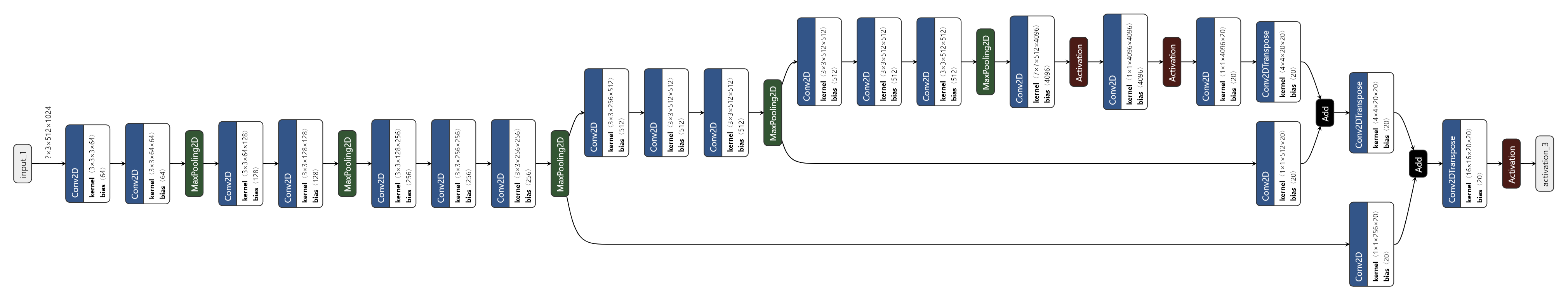
In this post, you use similar networks to run the ONNX workflow for semantic segmentation. The network consists of a VGG16-based encoder and three upsampling layers implemented using a deconvolutional layer. The network is trained in about 40,000 iterations on the Cityscapes Dataset.
There are multiple ways of converting the TensorFlow model to an ONNX file. One way is the one explained in the ResNet50 section. Keras also has its own Keras-to-ONNX file converter. Sometimes, some of the layers are not supported in the TensorFlow-to-ONNX but they are supported in the Keras to ONNX converter. Depending on the Keras framework and the type of layers used, you may need to choose between converters.
In the following code example, you directly convert the Keras model to ONNX using the Keras-to-ONNX converter. Download the pretrained semantic segmentation file, semantic_segmentation.hdf5.
import keras
import tensorflow as tf
from keras2onnx import convert_keras

def keras_to_onnx(model, output_filename):
   onnx = convert_keras(model, output_filename)
   with open(output_filename, "wb") as f:
       f.write(onnx.SerializeToString())

semantic_model = keras.models.load_model('/path/to/semantic_segmentation.hdf5')
keras_to_onnx(semantic_model, 'semantic_segmentation.onnx')
Figure 2 shows the architecture of the network.
Figure 2. The VGG16-based semantic segmentation model.
As in the previous example, use the following code example to create the engine for semantic segmentation.
import engine as eng
from onnx import ModelProto
import tensorrt as trt


engine_name = 'semantic.plan'
onnx_path = "semantic.onnx"
batch_size = 1

model = ModelProto()
with open(onnx_path, "rb") as f:
  model.ParseFromString(f.read())

d0 = model.graph.input[0].type.tensor_type.shape.dim[1].dim_value
d1 = model.graph.input[0].type.tensor_type.shape.dim[2].dim_value
d2 = model.graph.input[0].type.tensor_type.shape.dim[3].dim_value
shape = [batch_size , d0, d1 ,d2]
engine = eng.build_engine(onnx_path, shape= shape)
eng.save_engine(engine, engine_name)
To test the output of the model, use the Cityscapes Dataset. To work with Cityscapes, you must have the following functions: sub_mean_chw and color_map.
In the following code example, sub_mean_chw is for subtracting the mean value from the image as the preprocessing step and color_map is the mapping from the class ID to a color. The latter is used for visualization.
import numpy as np
from PIL import Image
import tensorrt as trt
import labels # from cityscapes evaluation scriptimport skimage.transform
TRT_LOGGER = trt.Logger(trt.Logger.WARNING)
trt_runtime = trt.Runtime(TRT_LOGGER)
MEAN = (71.60167789, 82.09696889, 72.30508881)
CLASSES = 20
HEIGHT = 512
WIDTH = 1024
def sub_mean_chw(data):
data = data.transpose((1, 2, 0)) # CHW -> HWCdata -= np.array(MEAN) # Broadcast subtractdata = data.transpose((2, 0, 1)) # HWC -> CHWreturn data
def rescale_image(image, output_shape, order=1):
image = skimage.transform.resize(image, output_shape,
order=order, preserve_range=True, mode='reflect')
return image
def color_map(output):
output = output.reshape(CLASSES, HEIGHT, WIDTH)
out_col = np.zeros(shape=(HEIGHT, WIDTH), dtype=(np.uint8, 3))
for x in range(WIDTH):
for y in range(HEIGHT):
if (np.argmax(output[:, y, x] )== 19):
out_col[y,x] = (0, 0, 0)
else:
out_col[y, x] = labels.id2label[labels.trainId2label[np.argmax(output[:, y, x])].id].color
return out_col
The following code example is the rest of the code for the previous example. You must run the previous block first because you need the defined functions. Use the example to compare the output of the Keras model and TensorRT engine semantic .plan file and then visualize both outputs. Replace the placeholders /path/to/semantic_segmentation.hdf5 and input_file_path as appropriate.
import engine as eng
import inference as inf
import keras
import tensorrt as trt

input_file_path = ‘munster_000172_000019_leftImg8bit.png’
onnx_file = "semantic.onnx"
serialized_plan_fp32 = "semantic.plan"
HEIGHT = 512
WIDTH = 1024

image = np.asarray(Image.open(input_file_path))
img = rescale_image(image, (512, 1024),order=1)
im = np.array(img, dtype=np.float32, order='C')
im = im.transpose((2, 0, 1))
im = sub_mean_chw(im)

engine = eng.load_engine(trt_runtime, serialized_plan_fp32)
h_input, d_input, h_output, d_output, stream = inf.allocate_buffers(engine, 1, trt.float32)
out = inf.do_inference(engine, im, h_input, d_input, h_output, d_output, stream, 1, HEIGHT, WIDTH)
out = color_map(out)

colorImage_trt = Image.fromarray(out.astype(np.uint8))
colorImage_trt.save(“trt_output.png”)

semantic_model = keras.models.load_model('/path/to/semantic_segmentation.hdf5')
out_keras= semantic_model.predict(im.reshape(-1, 3, HEIGHT, WIDTH))

out_keras = color_map(out_keras)
colorImage_k = Image.fromarray(out_keras.astype(np.uint8))
colorImage_k.save(“keras_output.png”)
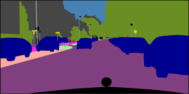
Figure 3 shows the actual image and the ground truth, and the output of Keras versus the output of the TensorRT engine. As you can see, the output for the TensorRT engine is similar to the one for Keras.
Figure 3a. Original image.
Figure 3b. Ground truth label.
Figure 3c. Output of TensorRT.
Figure 3d. Output of Keras.
Try it on other networks
Now you can try the ONNX workflow on other networks. For more information about good examples of segmentation networks, see Segmentation models with pretrained backbones on GitHub.
As an example, we show how to use the ONNX workflow with other networks. The network in this example is U-Net from the segmentation_models library. Here, we only loaded the model and did not train it. You may need to train these models on your preferred dataset.
One important point about these networks is that when you load these networks, their input layer sizes are as follows: (None, None, None, 3). To create a TensorRT engine, you need an ONNX file with a known input size. Before you convert this model to ONNX, change the network by assigning the size to its input and then convert it to the ONNX format.
As an example, load the U-Net network from this library (segmentation_models) and assign the size (244, 244, 3) to its input. After creating the TensorRT engine for the inference, do a similar conversion to what you did for semantic segmentation. Depending on the application and dataset, you may need to have a different color mapping.
# Requirement for TensorFlow 2
pip install tensorflow-gpu==2.1.0

# Other requirements
pip install -U segmentation-models
import segmentation_models as sm
import keras
from keras2onnx import convert_keras
from engine import *
onnx_path = 'unet.onnx'
engine_name = 'unet.plan'
batch_size = 1
CHANNEL = 3
HEIGHT = 224
WIDTH = 224

model = sm.Unet()
model._layers[0].batch_input_shape = (None, 224,224,3)
model = keras.models.clone_model(model)

onx = convert_keras(model, onnx_path)
with open(onnx_path, "wb") as f:
  f.write(onx.SerializeToString())

shape = [batch_size , HEIGHT, WIDTH, CHANNEL]
engine = build_engine(onnx_path, shape= shape)
save_engine(engine, engine_name)
As we mentioned earlier in this post, another way of downloading pretrained models is to download them from NVIDIA NGC Models. It has a list of checkpoints for pretrained models. As an example, you can search for UNet for TensorFlow and then go to the Download page to get the latest checkpoint.
Conclusion
In this post, we explained how to deploy deep learning applications using a TensorFlow-to-ONNX-to-TensorRT workflow, with several examples. The first example was ONNX-TensorRT on ResNet-50, and the second example was VGG16-based semantic segmentation that was trained on the Cityscapes Dataset. At the end of the post, we demonstrated how to apply this workflow on other networks. For more information about the best performance of training and inference, see NVIDIA Data Center Deep Learning Product Performance.
Hi all, I am currently trying to implement faster rcnn using tensorflow. Due to the limitations of the machine I am working on I can only use tensorflow 1.15. However, the model that I wanted to originally use as a feature extractor is built with Keras and tf2. Now I’m left wondering what I’m supposed to use to build the model for the feature extractor if I can’t use Keras. Should I just try to implement the inception resnet model by myself? Any help would be appreciated


 Solving a mystery that stumped scientists for decades, last November a group of computational biologists from Alphabet’s DeepMind used AI to predict a protein’s structure from its amino acid sequence. Not even a year later, a new study offers a more powerful model, capable of computing protein structures in as little as 10 minutes, on …
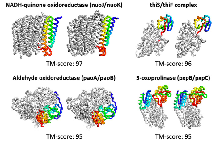
 Today, in partnership with NVIDIA, Google Cloud announced Dataflow is bringing GPUs to the world of big data processing to unlock new possibilities. With Dataflow GPU, users can now leverage the power of NVIDIA GPUs in their machine learning inference workflows. Here we show you how to access these performance benefits with BERT. Google Cloud’s Dataflow …
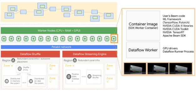
 We’ve been counting down to the release of Ray Tracing Gems II by providing early releases of select chapters once every week in July. This week’s chapter presents two real-time techniques for rendering caustics effects with ray tracing.
 This post was updated July 20, 2021 to reflect NVIDIA TensorRT 8.0 updates. In this post, you learn how to deploy TensorFlow trained deep learning models using the new TensorFlow-ONNX-TensorRT workflow. This tutorial uses NVIDIA TensorRT 8.0.0.3 and provides two code samples, one for TensorFlow v1 and one for TensorFlow v2. TensorRT is an inference …
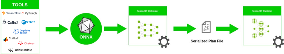


