Posted by Diego Martin Arroyo, Software Engineer and Federico Tombari, Research Scientist, Google Research
Information in a written document is not only conveyed by the meaning of the words contained in it, but also by the overall document layout. Layouts are commonly used to direct the order in which the reader parses a document to enable a better understanding (e.g., with columns or paragraphs), to provide helpful summaries (e.g., with titles) or for aesthetic purposes (e.g., when displaying advertisements).
While these design rules are easy to follow, it is difficult to explicitly define them without quickly needing to include exceptions or encountering ambiguous cases. This makes the automation of document design difficult, as any system with a hardcoded set of production rules will either be overly simplistic and thus incapable of producing original layouts (causing a lack of diversity in the layout of synthesized data), or too complex, with a large set of rules and their accompanying exceptions. In an attempt to solve this challenge, some have proposed machine learning (ML) techniques to synthesize document layouts. However, most ML-based solutions for automatic document design do not scale to a large number of layout components, or they rely on additional information for training, such as the relationships between the different components of a document.
In “Variational Transformer Networks for Layout Generation”, to be presented at CVPR 2021, we create a document layout generation system that scales to an arbitrarily large number of elements and does not require any additional information to capture the relationships between design elements. We use self-attention layers as building blocks of a variational autoencoder (VAE), which is able to model document layout design rules as a distribution, rather than using a set of predetermined heuristics, increasing the diversity of the generated layouts. The resulting Variational Transformer Network (VTN) model is able to extract meaningful relationships between the layout elements (paragraphs, tables, images, etc.), resulting in realistic synthetic documents (e.g., better alignment and margins). We show the effectiveness of this combination across different domains, such as scientific papers, UI layouts, and even furniture arrangements.
VAEs for Layout Generation
The ultimate goal of this system is to infer the design rules for a given type of layout from a collection of examples. If one considers these design rules as the distribution underlying the data, it is possible to use probabilistic models to discover it. We propose doing this with a VAE (widely used for tasks like image generation or anomaly detection), an autoencoder architecture that consists of two distinct subparts, the encoder and decoder. The encoder learns to compress the input to fewer dimensions, retaining only the necessary information to reconstruct the input, while the decoder learns to undo this operation. The compressed representation (also called the bottleneck) can be forced to behave like a known distribution (e.g., a uniform Gaussian). Feeding samples from this a priori distribution to the decoder segment of the network results in outputs similar to the training data.
An additional advantage of the VAE formulation is that it is agnostic to the type of operations used to implement the encoder and decoder segments. As such, we use self-attention layers (typically seen in Transformer architectures) to automatically capture the influence that each layout element has over the rest.
Transformers use self-attention layers to model long, sequenced relationships, often applied to an array of natural language understanding tasks, such as translation and summarization, as well as beyond the language domain in object detection or document layout understanding tasks. The self-attention operation relates every element in a sequence to every other and determines how they influence each other. This property is ideal to model relationships across different elements in a layout without the need for explicit annotations.
In order to synthesize new samples from these relationships, some approaches for layout generation [e.g., 1] and even for other domains [e.g., 2, 3] rely on greedy search algorithms, such as beam search, nucleus sampling or top-k sampling. Since these strategies are often based on exploration rules that tend to favor the most likely outcome at every step, the diversity of the generated samples is not guaranteed. However, by combining self-attention with the VAE’s probabilistic techniques, the model is able to directly learn a distribution from which it can extract new elements.
Modeling the Variational Bottleneck
The bottleneck of a VAE is commonly modeled as a vector representing the input. Since self-attention layers are a sequence-to-sequence architecture, i.e., a sequence of n input elements is mapped onto n output elements, the standard VAE formulation is difficult to apply. Inspired by BERT, we append an auxiliary token to the beginning of the sequence and treat it as the autoencoder bottleneck vector z. During training, the vector associated with this token is the only piece of information passed to the decoder, so the encoder needs to learn how to compress the entire document information in this vector. The decoder then learns to infer the number of elements in the document as well as the locations of each element in the input sequence from this vector alone. This strategy allows us to use standard techniques to regularize the bottleneck, such as the KL divergence.
Decoding
In order to synthesize documents with varying numbers of elements, the network needs to model sequences of arbitrary length, which is not trivial. While self-attention enables the encoder to adapt automatically to any number of elements, the decoder segment does not know the number of elements in advance. We overcome this issue by decoding sequences in an autoregressive way — at every step, the decoder produces an element, which is concatenated to the previously decoded elements (starting with the bottleneck vector z as input), until a special stop element is produced.
 |
| A visualization of our proposed architecture |
Turning Layouts into Input Data
A document is often composed of several design elements, such as paragraphs, tables, images, titles, footnotes, etc. In terms of design, layout elements are often represented by the coordinates of their enclosing bounding boxes. To make this information easily digestible for a neural network, we define each element with four variables (x, y, width, height), representing the element’s location on the page (x, y) and size (width, height).
Results
We evaluate the performance of the VTN following two criteria: layout quality and layout diversity. We train the model on publicly available document datasets, such as PubLayNet, a collection of scientific papers with layout annotations, and evaluate the quality of generated layouts by quantifying the amount of overlap and alignment between elements. We measure how well the synthetic layouts resemble the training distribution using the Wasserstein distance over the distributions of element classes (e.g., paragraphs, images, etc.) and bounding boxes. In order to capture the layout diversity, we find the most similar real sample for each generated document using the DocSim metric, where a higher number of unique matches to the real data indicates a more diverse outcome.
We compare the VTN approach to previous works like LayoutVAE and Gupta et al. The former is a VAE-based formulation with an LSTM backbone, whereas Gupta et al. use a self-attention mechanism similar to ours, combined with standard search strategies (beam search). The results below show that LayoutVAE struggles to comply with design rules, like strict alignments, as in the case of PubLayNet. Thanks to the self-attention operation, Gupta et al. can model these constraints much more effectively, but the usage of beam search affects the diversity of the results.
| |
IoU |
Overlap |
Alignment |
Wasserstein Class ↓ |
Wasserstein Box ↓ |
# Unique Matches ↑ |
| LayoutVAE |
0.171 |
0.321 |
0.472 |
– |
0.045 |
241 |
| Gupta et al. |
0.039 |
0.006 |
0.361 |
0.018 |
0.012 |
546 |
| VTN |
0.031 |
0.017 |
0.347 |
0.022 |
0.012 |
697 |
| Real Data |
0.048 |
0.007 |
0.353 |
– |
– |
– |
| Results on PubLayNet. Down arrows (↓) indicate that a lower score is better, whereas up arrows (↑) indicate higher is better. |
We also explore the ability of our approach to learn design rules in other domains, such as Android UIs (RICO), natural scenes (COCO) and indoor scenes (SUN RGB-D). Our method effectively learns the design rules of these datasets and produces synthetic layouts of similar quality as the current state of the art and a higher degree of diversity.
| |
IoU |
Overlap |
Alignment |
Wasserstein Class ↓ |
Wasserstein Box ↓ |
# Unique Matches ↑ |
| LayoutVAE |
0.193 |
0.400 |
0.416 |
– |
0.045 |
496 |
| Gupta et al. |
0.086 |
0.145 |
0.366 |
0.004 |
0.023 |
604 |
| VTN |
0.115 |
0.165 |
0.373 |
0.007 |
0.018 |
680 |
| Real Data |
0.084 |
0.175 |
0.410 |
– |
– |
– |
| Results on RICO. Down arrows (↓) indicate that a lower score is better, whereas up arrows (↑) indicate higher is better. |
| |
IoU |
Overlap |
Alignment |
Wasserstein Class ↓ |
Wasserstein Box ↓ |
# Unique Matches ↑ |
| LayoutVAE |
0.325 |
2.819 |
0.246 |
– |
0.062 |
700 |
| Gupta et al. |
0.194 |
1.709 |
0.334 |
0.001 |
0.016 |
601 |
| VTN |
0.197 |
2.384 |
0.330 |
0.0005 |
0.013 |
776 |
| Real Data |
0.192 |
1.724 |
0.347 |
– |
– |
– |
| Results for COCO. Down arrows (↓) indicate that a lower score is better, whereas up arrows (↑) indicate higher is better. |
Below are some examples of layouts produced by our method compared to existing methods. The design rules learned by the network (location, margins, alignment) resemble those of the original data and show a high degree of variability.
| LayoutVAE |
|
| Gupta et al. |
|
| VTN |
|
| Qualitative results of our method on PubLayNet compared to existing state-of-the-art methods. |
Conclusion
In this work we show the feasibility of using self-attention as part of the VAE formulation. We validate the effectiveness of this approach for layout generation, achieving state-of-the-art performance on various datasets and across different tasks. Our research paper also explores alternative architectures for the integration of self-attention and VAEs, exploring non-autoregressive decoding strategies and different types of priors, and analyzes advantages and disadvantages. The layouts produced by our method can help to create synthetic training data for downstream tasks, such as document parsing or automating graphic design tasks. We hope that this work provides a foundation for continued research in this area, as many subproblems are still not completely solved, such as how to suggest styles for the elements in the layout (text font, which image to choose, etc.) or how to reduce the amount of training data necessary for the model to generalize.
AcknowledgementsWe thank our co-author Janis Postels, as well as Alessio Tonioni and Luca Prasso for helping with the design of several of our experiments. We also thank Tom Small for his help creating the animations for this post.


 The most commonly diagnosed cancer in the US today is skin cancer. There are three main variants: melanoma, basal cell carcinoma (BCC), and squamous cell carcinoma (SCC). Though melanoma only accounts for roughly 1% of all skin cancers, it is the most fatal, metastasizing rapidly without early detection and treatment. This makes early detection critical, … Continued
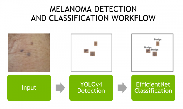
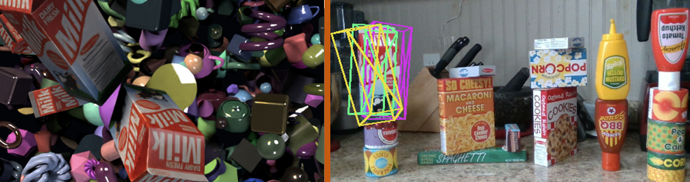
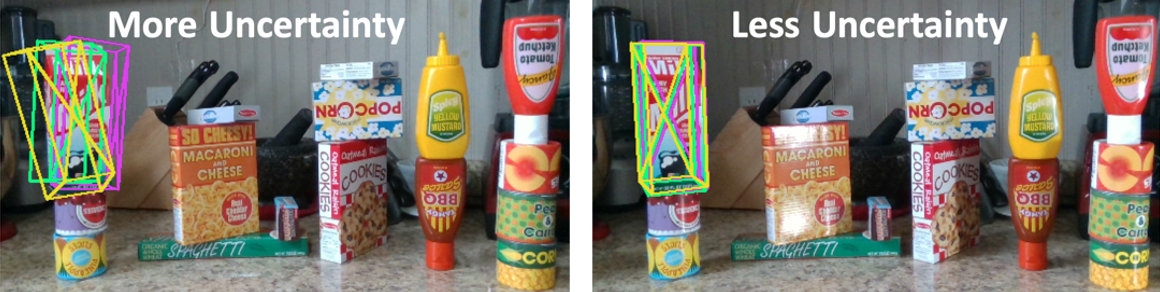
 Researchers from NVIDIA, University of Texas at Austin and Caltech developed a simple, efficient, and plug-and-play uncertainty quantification method for the 6-DoF object pose estimation task, using an ensemble of K pre-trained estimators with different architectures and/or training data sources.
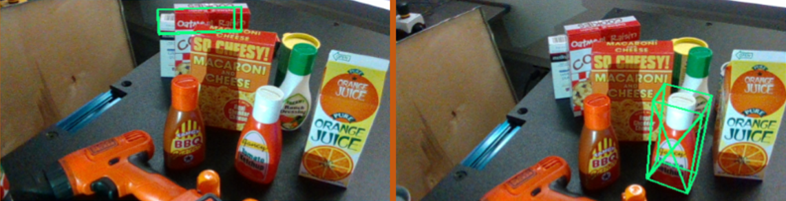


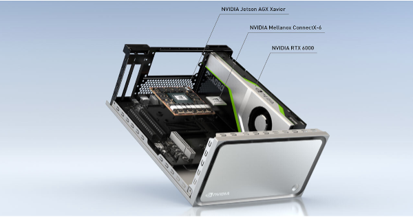
 NVIDIA RTX ray tracing has transformed graphics and rendering. With powerful software applications like Luxion KeyShot, more users can take advantage of RTX technology to speed up graphic workflows — like rendering caustics.