Posted by Maxim Tabachnyk, Staff Software Engineer and Stoyan Nikolov, Senior Engineering Manager, Google Research
The increasing complexity of code poses a key challenge to productivity in software engineering. Code completion has been an essential tool that has helped mitigate this complexity in integrated development environments (IDEs). Conventionally, code completion suggestions are implemented with rule-based semantic engines (SEs), which typically have access to the full repository and understand its semantic structure. Recent research has demonstrated that large language models (e.g., Codex and PaLM) enable longer and more complex code suggestions, and as a result, useful products have emerged (e.g., Copilot). However, the question of how code completion powered by machine learning (ML) impacts developer productivity, beyond perceived productivity and accepted suggestions, remains open.
Today we describe how we combined ML and SE to develop a novel Transformer-based hybrid semantic ML code completion, now available to internal Google developers. We discuss how ML and SEs can be combined by (1) re-ranking SE single token suggestions using ML, (2) applying single and multi-line completions using ML and checking for correctness with the SE, or (3) using single and multi-line continuation by ML of single token semantic suggestions. We compare the hybrid semantic ML code completion of 10k+ Googlers (over three months across eight programming languages) to a control group and see a 6% reduction in coding iteration time (time between builds and tests) and a 7% reduction in context switches (i.e., leaving the IDE) when exposed to single-line ML completion. These results demonstrate that the combination of ML and SEs can improve developer productivity. Currently, 3% of new code (measured in characters) is now generated from accepting ML completion suggestions.
Transformers for Completion A common approach to code completion is to train transformer models, which use a self-attention mechanism for language understanding, to enable code understanding and completion predictions. We treat code similar to language, represented with sub-word tokens and a SentencePiece vocabulary, and use encoder-decoder transformer models running on TPUs to make completion predictions. The input is the code that is surrounding the cursor (~1000-2000 tokens) and the output is a set of suggestions to complete the current or multiple lines. Sequences are generated with a beam search (or tree exploration) on the decoder.
During training on Google’s monorepo, we mask out the remainder of a line and some follow-up lines, to mimic code that is being actively developed. We train a single model on eight languages (C++, Java, Python, Go, Typescript, Proto, Kotlin, and Dart) and observe improved or equal performance across all languages, removing the need for dedicated models. Moreover, we find that a model size of ~0.5B parameters gives a good tradeoff for high prediction accuracy with low latency and resource cost. The model strongly benefits from the quality of the monorepo, which is enforced by guidelines and reviews. For multi-line suggestions, we iteratively apply the single-line model with learned thresholds for deciding whether to start predicting completions for the following line.
Encoder-decoder transformer models are used to predict the remainder of the line or lines of code.
Re-rank Single Token Suggestions with ML While a user is typing in the IDE, code completions are interactively requested from the ML model and the SE simultaneously in the backend. The SE typically only predicts a single token. The ML models we use predict multiple tokens until the end of the line, but we only consider the first token to match predictions from the SE. We identify the top three ML suggestions that are also contained in the SE suggestions and boost their rank to the top. The re-ranked results are then shown as suggestions for the user in the IDE.
In practice, our SEs are running in the cloud, providing language services (e.g., semantic completion, diagnostics, etc.) with which developers are familiar, and so we collocated the SEs to run on the same locations as the TPUs performing ML inference. The SEs are based on an internal library that offers compiler-like features with low latencies. Due to the design setup, where requests are done in parallel and ML is typically faster to serve (~40 ms median), we do not add any latency to completions. We observe a significant quality improvement in real usage. For 28% of accepted completions, the rank of the completion is higher due to boosting, and in 0.4% of cases it is worse. Additionally, we find that users type >10% fewer characters before accepting a completion suggestion.
Check Single / Multi-line ML Completions for Semantic Correctness At inference time, ML models are typically unaware of code outside of their input window, and code seen during training might miss recent additions needed for completions in actively changing repositories. This leads to a common drawback of ML-powered code completion whereby the model may suggest code that looks correct, but doesn’t compile. Based on internal user experience research, this issue can lead to the erosion of user trust over time while reducing productivity gains.
We use SEs to perform fast semantic correctness checks within a given latency budget (<100ms for end-to-end completion) and use cached abstract syntax trees to enable a “full” structural understanding. Typical semantic checks include reference resolution (i.e., does this object exist), method invocation checks (e.g., confirming the method was called with a correct number of parameters), and assignability checks (to confirm the type is as expected).
For example, for the coding language Go, ~8% of suggestions contain compilation errors before semantic checks. However, the application of semantic checks filtered out 80% of uncompilable suggestions. The acceptance rate for single-line completions improved by 1.9x over the first six weeks of incorporating the feature, presumably due to increased user trust. As a comparison, for languages where we did not add semantic checking, we only saw a 1.3x increase in acceptance.
Language servers with access to source code and the ML backend are collocated on the cloud. They both perform semantic checking of ML completion suggestions.
Results With 10k+ Google-internal developers using the completion setup in their IDE, we measured a user acceptance rate of 25-34%. We determined that the transformer-based hybrid semantic ML code completion completes >3% of code, while reducing the coding iteration time for Googlers by 6% (at a 90% confidence level). The size of the shift corresponds to typical effects observed for transformational features (e.g., key framework) that typically affect only a subpopulation, whereas ML has the potential to generalize for most major languages and engineers.
Fraction of all code added by ML
2.6%
Reduction in coding iteration duration
6%
Reduction in number of context switches
7%
Acceptance rate (for suggestions visible for >750ms)
25%
Average characters per accept
21
Key metrics for single-line code completion measured in production for 10k+ Google-internal developers using it in their daily development across eight languages.
Fraction of all code added by ML (with >1 line in suggestion)
0.6%
Average characters per accept
73
Acceptance rate (for suggestions visible for >750ms)
34%
Key metrics for multi-line code completion measured in production for 5k+ Google-internal developers using it in their daily development across eight languages.
Providing Long Completions while Exploring APIs We also tightly integrated the semantic completion with full line completion. When the dropdown with semantic single token completions appears, we display inline the single-line completions returned from the ML model. The latter represent a continuation of the item that is the focus of the dropdown. For example, if a user looks at possible methods of an API, the inline full line completions show the full method invocation also containing all parameters of the invocation.
Integrated full line completions by ML continuing the semantic dropdown completion that is in focus.
Suggestions of multiple line completions by ML.
Conclusion and Future Work We demonstrate how the combination of rule-based semantic engines and large language models can be used to significantly improve developer productivity with better code completion. As a next step, we want to utilize SEs further, by providing extra information to ML models at inference time. One example can be for long predictions to go back and forth between the ML and the SE, where the SE iteratively checks correctness and offers all possible continuations to the ML model. When adding new features powered by ML, we want to be mindful to go beyond just “smart” results, but ensure a positive impact on productivity.
Acknowledgements This research is the outcome of a two-year collaboration between Google Core and Google Research, Brain Team. Special thanks to Marc Rasi, Yurun Shen, Vlad Pchelin, Charles Sutton, Varun Godbole, Jacob Austin, Danny Tarlow, Benjamin Lee, Satish Chandra, Ksenia Korovina, Stanislav Pyatykh, Cristopher Claeys, Petros Maniatis, Evgeny Gryaznov, Pavel Sychev, Chris Gorgolewski, Kristof Molnar, Alberto Elizondo, Ambar Murillo, Dominik Schulz, David Tattersall, Rishabh Singh, Manzil Zaheer, Ted Ying, Juanjo Carin, Alexander Froemmgen and Marcus Revaj for their contributions.
NVIDIA Math Libraries are available to boost your application’s performance, from GPU-accelerated implementations of BLAS to random number generation.
There are three main ways to accelerate GPU applications: compiler directives, programming languages, and preprogrammed libraries. Compiler directives such as OpenACC aIlow you to smoothly port your code to the GPU for acceleration with a directive-based programming model. While it is simple to use, it may not provide optimal performance in certain scenarios.
Programming languages such as CUDA C and C++ give you greater flexibility when accelerating your applications, but it is also the user’s responsibility to write code that takes advantage of new hardware features to achieve optimal performance on the latest hardware. This is where preprogrammed libraries fill in the gap.
In addition to enhancing code reusability, the NVIDIA Math Libraries are optimized to make best use of GPU hardware for the greatest performance gain. If you’re looking for a straightforward way to speed up your application, continue reading to learn about using libraries to improve your application’s performance.
The NVIDIA math libraries, available as part of the CUDA Toolkit and the high-performance computing (HPC) software development kit (SDK), offer high-quality implementations of functions encountered in a wide range of compute-intensive applications. These applications include the domains of machine learning, deep learning, molecular dynamics, computational fluid dynamics (CFD), computational chemistry, medical imaging, and seismic exploration.
These libraries are designed to replace the common CPU libraries such as OpenBLAS, LAPACK, and Intel MKL, as well as accelerate applications on NVIDIA GPUs with minimal code changes. To show the process, we created an example of the double precision general matrix multiplication (DGEMM) functionality to compare the performance of cuBLAS with OpenBLAS.
The code example below demonstrates the use of the OpenBLAS DGEMM call.
// Init Data
…
// Execute GEMM
cblas_dgemm(CblasColMajor, CblasNoTrans, CblasTrans, m, n, k, alpha, A.data(), lda, B.data(), ldb, beta, C.data(), ldc);
Code example 2 below shows the cuBLAS dgemm call.
// Init Data
…
// Data movement to GPU
…
// Execute GEMM
cublasDgemm(cublasH, CUBLAS_OP_N, CUBLAS_OP_T, m, n, k, &alpha, d_A, lda, d_B, ldb, &beta, d_C, ldc));
As shown in the example above, you can simply add and replace the OpenBLAS CPU code with the cuBLAS API functions. See the full code for both the cuBLAS and OpenBLAS examples. This cuBLAS example was run on an NVIDIA(R) V100 Tensor Core GPU with a nearly 20x speed-up. The graph below displays the speedup and specs when running these examples.
Figure 1. Replacing the OpenBLAS CPU code with the cuBLAS API function on the GPU yields a 19.2x speed-up in the DGEMM computation, where A, B, and C matrices are 4K x 4K matrices, on the CPU and the GPU.
Fun fact: These libraries are invoked in the higher-level Python APIs such as cuPy, cuDNN and RAPIDS, so if you have experience with those, then you have already been using these NVIDIA Math Libraries.
Delivering better performance compared to CPU-only alternatives
There are many NVIDIA Math Libraries to take advantage of, from GPU-accelerated implementations of BLAS to random number generation. Take a look below at an overview of the NVIDIA Math Libraries and learn how to get started to easily boost your application’s performance.
Speed up Basic Linear Algebra Subprograms with cuBLAS
General Matrix Multiplication (GEMM) is one of the most popular Basic Linear Algebra Subprograms (BLAS) deployed in AI and scientific computing. GEMMs also form the foundational blocks for deep learning frameworks. To learn more about the use of GEMMs in deep learning frameworks, see Why GEMM Is at the Heart of Deep Learning.
The cuBLAS Library is an implementation of BLAS which leverages GPU capabilities to achieve great speed-ups. It comprises routines for performing vector and matrix operations such as dot products (Level 1), vector addition (Level 2), and matrix multiplication (Level 3).
Additionally, if you would like to parallelize your matrix-matrix multiplies, cuBLAS supports the versatile batched GEMMs which finds use in tensor computations, machine learning, and LAPACK. For more details about improving efficiency in machine learning and tensor contractions, see Tensor Contractions with Extended BLAS Kernels on CPU and GPU.
cuBLASXt
If the problem size is too big to fit on the GPU, or your application needs single-node, multi-GPU support, cuBLASXt is a great option. cuBLASXt allows for hybrid CPU-GPU computation and supports BLAS Level 3 operations that perform matrix-to-matrix operations such as herk which performs the Hermitian rank update.
cuBLASLt
cuBLASLt is a lightweight library that covers GEMM. cuBLASLt uses fused kernels to speed up applications by “combining” two or more kernels into a single kernel which allows for reuse of data and reduced data movement. cuBLASLt also allows users to set the post-processing options for the epilogue (apply Bias and then ReLU transform or apply bias gradient to an input matrix).
cuBLASMg: CUDA Math Library Early Access Program
For large-scale problems, check out cuBLASMg for state-of-the-art multi-GPU, multi-node matrix-matrix multiplication support. It is currently a part of the CUDA Math Library Early Access Program. Apply for access.
Process sparse matrices with cuSPARSE
Sparse-matrix, dense-matrix multiplication (SpMM) is fundamental to many complex algorithms in machine learning, deep learning, CFD, and seismic exploration, as well as economic, graph, and data analytics. Efficiently processing sparse matrices is critical to many scientific simulations.
The growing size of neural networks and the associated increase in cost and resources incurred has led to the need for sparsification. Sparsity has gained popularity in the context of both deep learning training and inference to optimize the use of resources. For more insight into this school of thought and the need for a library such as cuSPARSE, see The Future of Sparsity in Deep Neural Networks.
cuSPARSE provides a set of basic linear algebra subprograms used for handling sparse matrices which can be used to build GPU-accelerated solvers. There are four categories of the library routines:
Level 1 operates between a sparse vector and dense vector, such as the dot product between two vectors.
Level 2 operates between a sparse matrix and a dense vector, such as a matrix-vector product.
Level 3 operates between a sparse matrix and a set of dense vectors, such as a matrix-matrix product).
Level 4 allows conversion between different matrix formats and compression of compressed sparse row (CSR) matrices.
cuSPARSELt
For a lightweight version of the cuSPARSE library with compute capabilities to perform sparse matrix-dense matrix multiplication along with helper functions for pruning and compression of matrices, try cuSPARSELt. For a better understanding of the cuSPARSELt library, see Exploiting NVIDIA Ampere Structured Sparsity with cuSPARSELt.
Accelerate tensor applications with cuTENSOR
The cuTENSOR library is a tensor linear algebra library implementation. Tensors are core to machine learning applications and are an essential mathematical tool used to derive the governing equations for applied problems. cuTENSOR provides routines for direct tensor contractions, tensor reductions, and element-wise tensor operations. cuTENSOR is used to improve performance in deep learning training and inference, computer vision, quantum chemistry, and computational physics applications.
cuTENSORMg
If you still want cuTENSOR features, but with support for large tensors that can be distributed across multi-GPUs in a single node such as with the DGX A100, cuTENSORMg is the library of choice. It provides broad mixed-precision support, and its main computational routines include direct tensor contractions, tensor reductions, and element-wise tensor operations.
GPU-accelerated LAPACK features with cuSOLVER
The cuSOLVER library is a high-level package useful for linear algebra functions based on the cuBLAS and cuSPARSE libraries. cuSOLVER provides LAPACK-like features, such as matrix factorization, triangular solve routines for dense matrices, a sparse least-squares solver, and an eigenvalue solver.
There are three separate components of cuSOLVER:
cuSolverDN is used for dense matrix factorization.
cuSolverSP provides a set of sparse routines based on sparse QR factorization.
cuSolverRF is a sparse re-factorization package, useful for solving sequences of matrices with a shared sparsity pattern.
cuSOLVERMg
For GPU-accelerated ScaLAPACK features, a symmetric eigensolver, 1-D column block cyclic layout support, and single-node, multi-GPU support for cuSOLVER features, consider cuSOLVERMg.
cuSOLVERMp
Multi-node, multi-GPU support is needed for solving large systems of linear equations. Known for its lower-upper factorization and Cholesky factorization features, cuSOLVERMp is a great solution.
Large-scale generation of random numbers with cuRAND
The cuRAND library focuses on the generation of random numbers through pseudo-random or quasi-random number generators on either the host (CPU) API or a device (GPU) API. The host API can generate random numbers purely on the host and store them in host memory, or they can be generated on the device where the calls to the library happen on the host, but the random number generation occurs on the device and is stored to global memory.
The device API defines functions for setting up random number generator states and generating sequences of random numbers which can be immediately used by user kernels without having to read and write to global memory. Several physics-based problems have shown the need for large-scale random number generation.
cuFFT, the CUDA Fast Fourier Transform (FFT) library provides a simple interface for computing FFTs on an NVIDIA GPU. The FFT is a divide-and-conquer algorithm for efficiently computing discrete Fourier transforms of complex or real-valued data sets. It is one of the most widely used numerical algorithms in computational physics and general signal processing.
cuFFT can be used for a wide range of applications, including medical imaging and fluid dynamics. Parallel Computing for Quantitative Blood Flow Imaging in Photoacoustic Microscopy illustrates the use of cuFFT in physics-based applications. Users with existing FFTW applications should use cuFFTW to easily port code to NVIDIA GPUs with minimal effort. The cuFFTW library provides the FFTW3 API to facilitate porting of existing FFTW applications.
cuFFTXt
To distribute FFT calculations across GPUs in a single node, check out cuFFTXt. This library includes functions to help users manipulate data on multiple GPUs and keep track of data ordering, which allows data to be processed in the most efficient way possible.
cuFFTMp
Not only is there multi-GPU support within a single system, cuFFTMp provides support for multi-GPUs across multiple nodes. This library can be used with any MPI application since it is independent of the quality of MPI implementation. It uses NVSHMEM which is a communication library based on OpenSHMEM standards that was designed for NVIDIA GPUs.
cuFFTDx
To improve performance by avoiding unnecessary trips to global memory and allowing fusion of FFT kernels with other operations, check out cuFFT device extensions (cuFFTDx) . Part of the Math Libraries Device Extensions, it allows applications to compute FFTs inside user kernels.
Optimize standard mathematical functions with CUDA Math API
The CUDA Math API is a collection of standard mathematical functions optimized for every NVIDIA GPU architecture. All of the CUDA libraries rely on the CUDA Math Library. CUDA Math API supports all C99 standard float and double math functions, float, double, and all rounding modes, and different functions such as trigonometry and exponential functions ( cospi, sincos) and additional inverse error functions (erfinv, erfcinv).
Customize code using C++ templates with CUTLASS
Matrix multiplications are the foundation of many scientific computations. These multiplications are particularly important in efficient implementation of deep learning algorithms. Similar to cuBLAS, CUDA Templates for Linear Algebra Subroutines (CUTLASS) comprises a set of linear algebra routines to carry out efficient computation and scaling.
It incorporates strategies for hierarchical decomposition and data movement similar to those used to implement cuBLAS and cuDNN. However, unlike cuBLAS, CUTLASS is increasingly modularized and reconfigurable. It decomposes the moving parts of GEMM into fundamental components or blocks available as C++ template classes, thereby giving you flexibility to customize your algorithms.
The software is pipelined to hide latency and maximize data reuse. Access shared memory without conflict to maximize your data throughput, eliminate memory footprints, and design your application exactly the way you want. To learn more about using CUTLASS to improve the performance of your application, see CUTLASS: Fast Linear Algebra in CUDA C++.
Compute differential equations with AmgX
AmgX provides a GPU-accelerated AMG (algebraic multi-grid) library and is supported on a single GPU or multi-GPUs on distributed nodes. It allows users to create complex nested solvers, smoothers, and preconditioners. This library implements classical and aggregation-based algebraic multigrid methods with different smoothers such as block-Jacobi, Gauss-Seidel, and dense LU.
This library also contains preconditioned Krylov subspace iterative methods such as PCG and BICGStab. AmgX provides up to 10x acceleration to the computationally intense linear solver portion of simulations and is well-suited for implicit unstructured methods.
AmgX was specifically developed for CFD applications and can be used in domains such as energy, physics, and nuclear safety. A real-life example of the AmgX library is in solving the Poisson Equation for small-scale to large-scale computing problems.
The flying snake simulation example shows the reduction in time and cost incurred when using the AmgX wrapper on GPUs to accelerate CFD codes. There is a 21x speed-up with 3 million mesh points on one K20 GPU when compared to one 12-core CPU node.
Get started with NVIDIA Math Libraries
cuBLAS, cuRAND, cuFFT, cuSPARSE, cuSOLVER, and the CUDA Math Library are included in both the NVIDIA HPC SDK and the CUDA Toolkit
The Math Library Device Extensions (cuFFTDx) are available in MathDx 20.22
We continue working to improve the NVIDIA Math Libraries. If you have questions or a new feature request, contact Product Manager Matthew Nicely.
Acknowledgements
We would like to thank Matthew Nicely for his guidance and active feedback. A special thank you to Anita Weemaes for all her feedback and her continued support throughout.
How is speech AI related to AI, ML and DL? A quick guide on need-to-know speech AI terminologies like automatic speech recognition and text-to-speech.
Speech AI is the technology that makes it possible to communicate with computer systems using your voice. Commanding an in-car assistant or handling a smart home device? An AI-enabled voice interface helps you interact with devices without having to type or tap on a screen.
The field of speech AI is relatively new. But as voice interaction matures and expands to new devices and platforms, it’s important for developers to keep up with the evolving terminology.
In this explainer, I present key concepts from the world of speech AI, describe where it is situated in the bigger universe of AI, and discuss how it relates to other fields of science and technology.
Foundational concepts
You might have heard of, or even be familiar with these technologies but for the sake of completeness, here are the basics:
Artificial intelligence (AI) refers to the broad discipline of creating intelligent machines that either match or exceed human-level cognitive abilities.
Machine learning (ML) is a subfield of AI that involves creating methods and systems that learn how to carry out specific tasks using past data.
How are speech AI systems related to AI, ML, and DL?
Speech AI is the use of AI for voice-based technologies. Core components of a speech AI system include:
An automatic speech recognition (ASR) system, also known as speech-to-text, speech recognition, or voice recognition. This converts the speech audio signal into text.
A text-to-speech (TTS) system, also known as speech synthesis. This turns a text into a verbal, audio form.
Speech AI is a subfield within conversational AI, drawing its techniques primarily from the fields of DL and ML. The relationship between AI, ML, DL, and speech AI can be represented by the Venn diagram in Figure 1.
Figure 1. The relationship between AI, ML, DL, and speech AI
Figure 1 shows that conversational AI is the larger universe of language-based applications, of which not all include a voice component (speech).
Here’s how speech AI technologies work side by side with other tools and techniques to form a complete conversational AI system.
Conversational AI
Conversational AI is the discipline that involves designing intelligent systems capable of interacting with human users through natural language in a conversational fashion. Commercial examples include home assistants and chatbots (for example, an insurance claim chatbot or travel agent chatbot).
There can be multiple modalities for conversation, including audio, text, and sign language but when the input and output are spoken natural language, you have a voice-based conversational AI system (Figure 2).
Figure 2. A voice-based conversational AI system
The components of a typical voice-based conversational AI system include the following:
A speech interface, enabled by speech AI technologies, enables the system to interact with users through a spoken natural-language format.
A dialog system manages the conversation with the user while interacting with external fulfillment systems to satisfy the user’s needs. It consists of two components:
A natural language understanding (NLU) module parses the text and identifies relevant information, such as the intent of the user, and any relevant parameter to that intent. For example, if the user is requesting, “What’s the weather tomorrow morning?”, then “weather information” is the intent, while time is a releva,nt parameter to extract from the request, which is “tomorrow morning” in this case.
NLU is part of natural language processing (NLP), a subfield of linguistics and artificial intelligence concerned with computational methods to process and analyze natural language data.
A dialog manager monitors the state of the conversation and decides which action to take next. The dialog manager takes information from the NLU module, remembers the context, and fulfills the user’s request.
The fulfillment engines execute the tasks that are functional to the conversational AI system, for instance: retrieving weather information, reading news, booking tickets, providing stock market information, answering trivia Q&A and much more. In general, they are not considered part of the conversational AI system, but work closely together to satisfy the user’s needs.
Speech AI concepts
In this section, we dive into concepts specific to speech AI: automatic speech recognition and text-to-speech.
Automatic speech recognition
A typical deep learning-based ASR pipeline includes five main components (Figure 3).
Figure 3. Anatomy of a deep learning-based ASR pipeline
Feature extractor
A feature extractor segments the audio signal into fixed-length blocks (aka. time step) and then converts the blocks from the temporal domain to the frequency domain.
Acoustic model
This machine learning model (usually a multi-layer deep neural network) predicts the probabilities over characters at each time step of the audio data.
Decoder and language model
A decoder converts the matrix of probabilities given by the acoustic model into a sequence of characters, which in turn make words and sentences.
A language model (LM) can give a score indicating the likelihood of a sentence appearing in its training corpus. For example, an LM trained on an English corpus will judge “Recognize speech” as more likely than “Wreck a nice peach,” while also judging “Je suis un étudiant” as quite unlikely (for that being a French sentence).
When coupled with an LM, a decoder would be able to correct what it “hears” (“I’ve got rose beef for lunch”) to what makes more common sense (“I’ve got roast beef for lunch”), for the LM will give a higher score for the latter sentence than the former.
Punctuation and capitalization model
The punctuation and capitalization model adds punctuations and capitalizes the decoder-produced text.
Inverse text normalization model
Lastly, inverse text normalization (ITN) rules are applied to transform the text in verbal format into a desired written format, for example, “ten o’clock” to “10:00,” or “ten dollars” to “$10”.
Other ASR concepts
Word error rate (WER) and character error rate (CER) are typical performance metrics of ASR systems.
WER is the number of errors divided by the total number of spoken words. For example, if there are five errors in a total of 50 spoken words, the WER would be 25%.
CER operates similarly except on characters instead of words. Languages like Japanese and Mandarin do not have “words” separated by a specific marker or delimiter (like spaces for English).
Figure 4. Anatomy of a two-stage deep-learning-based TTS pipeline
Text-to-speech (TTS)
The Text-to-speech step is commonly achieved using two different approaches:
A two-stage pipeline: Two separate networks are trained separately for converting speech-to-text: the spectrogram generator network and the vocoder network.
An end-to-end pipeline: Uses one model to generate audio straight from text.
The components of a two-state pipeline are:
Text normalization model: Transforms the text in written format into a verbal format, for example, “10:00” to “ten o’clock”, “$10” to “ten dollars”. This is the opposite process of ITN.
Spectrogram generator network: The first stage of the TTS pipeline uses a neural network to generate a spectrogram from text.
Vocoder network: The second stage of the TTS pipeline takes the spectrogram from the spectrogram generator network as an input and generates a natural-sounding speech.
Speech Synthesis Markup Language
Other TTS concepts include Speech Synthesis Markup Language (SSML), which is an XML-based markup language that lets you specify how input text is converted into synthesized speech. Your configuration can make the generated synthetic speech more expressive using parameters such as pitch, pronunciation, speaking rate, and volume.
Common SSML tags include the following:
Prosody is used to customize the pitch, speaking rate, and volume of the generated speech.
Phoneme is used to override manually the pronunciation of words in the generated synthetic voice.
Mean opinion score
To assess the quality of TTS engines, Mean opinion score (MOS) is frequently used. Originating from the telecommunications field, MOS is defined as the arithmetic mean over ratings given by human evaluators for a provided stimulus in a subjective quality evaluation test.
For example, a common TTS evaluation setup would be a group of people listening to generated samples and giving each sample a score from 0 to 5. MOS is then calculated as the average score of overall evaluators and test samples.
How to get started with speech AI
Speech AI has nowadays become mainstream and an integral part of consumers’ everyday life. Businesses are discovering new ways of bringing added value to their products by incorporating speech AI capabilities.
The best way to gain expertise in speech AI is to experience it. For more information about how to build and deploy real-time speech AI pipelines for your conversational AI application, see the free Building Speech AI Applications ebook.
Present barrier provides an easy way of synchronizing present calls between application windows on the same machine, as well as on distributed systems.
Swap groups and swap barriers are well-known methods to synchronize buffer swaps between different windows on the same system and on distributed systems, respectively. Initially introduced for OpenGL, they were later extended through public NvAPI interfaces and supported in DirectX 9 through 12.
NVIDIA now introduces the concept of present barriers. They combine swap groups and swap barriers and provide a simple way to set up synchronized present calls within and between systems.
When an application requests to join the present barrier, the driver tries to set up either a swap group or a combination of a swap group and a swap barrier, depending on the current system configuration. The functions are again provided through public NvAPI interfaces.
The present barrier is only effective when an application is in a full-screen state with no window borders, as well as no desktop scaling or taskbar composition. If at least one of these requirements is not met, the present barrier disengages and reverts to a pending state until they all are. When the present barrier is in the pending state, no synchronization across displays happens.
Similarly, the present barrier works correctly only when displays are attached to the same GPU and set to the same timing. Displays can also be synchronized with either the Quadro Sync card or the NVLink connector.
Display synchronization occurs in one of two ways:
The displays have been configured to form a synchronized group or synchronized to an external sync source, or both, using the Quadro Sync add-on board.
The displays have been synchronized by creating a Mosaic display surface spanning the displays.
When the display timings have been synchronized through one of these methods, then the DX12 present barrier is available to use.
NvAPI interfaces
To set up synchronized present calls through the present barrier extension in NvAPI, the app must make sure that the present barrier is supported at all. If that’s the case, it must create a present barrier client, register needed DirectX resources, and join the present barrier.
Query present barrier support
Before any attempt to synchronize present calls, the application should first check whether present barrier synchronization is supported on the current OS, driver, and hardware configuration. This is done by calling the according function with the desired D3D12 device as a parameter.
ID3D12Device* device;
... // initialize the device
bool supported;
assert(NvAPI_D3D12_QueryPresentBarrierSupport(device, &supported) == NVAPI_OK);
if(supported) {
  LOG("D3D12 present barrier is supported on this system.");
  ...
}
Create a present barrier client handle
If the system offers present barrier support, the app can create a present barrier client by supplying the D3D12 device and DXGI swap chain. The handle is used to register needed resources, join or leave the present barrier, and query frame statistics.
After client creation, the present barrier needs access to the swap chain’s buffer resources and a fence object for proper frame synchronization. The fence value is incremented by the present barrier at each frame and must not be changed by the app. However, the app may use it to synchronize command allocator usage between the host and device. The function must be called again whenever the swap chain’s buffers change.
ID3D12Fence pbFence; // the app may wait on the fence but must not signal it
assert(SUCCEEDED(device->CreateFence(0, D3D12_FENCE_FLAG_NONE, IID_PPV_ARGS(&pbFence))));
ID3D12Resource** backBuffers;
unsigned int backBufferCount;
... // query buffers from swap chain
assert(NvAPI_D3D12_RegisterPresentBarrierResources(pbClientHandle, pbFence, backBuffers, backBufferCount) == NVAPI_OK);
Join the present barrier
After creating the present barrier client handle and registering the scanout resources, the application can join present barrier synchronization. Future present calls are then synchronized with other clients.
When everything is set up, the app can execute its main loop without any changes, including the present call. The present barrier handles synchronization by itself. While the app can choose to use the fence provided to the present barrier for host and device synchronization, it is also practical to use its own dedicated one.
Query statistics
While the client is registered to the present barrier, the app can query frame and synchronization statistics at any time to make sure that everything works as intended.
The present barrier statistics object filled by the function call supplies several useful values.
SyncMode: The present barrier mode of the client from the last present call. Possible values:
PRESENT_BARRIER_NOT_JOINED: The client has not joined the present barrier.
PRESENT_BARRIER_SYNC_CLIENT: The client joined the present barrier but is not synchronized with any other clients.
PRESENT_BARRIER_SYNC_SYSTEM: The client joined the present barrier and is synchronized with other clients within the system.
PRESENT_BARRIER_SYNC_CLUSTER: The client joined the present barrier and is synchronized with other clients within the system and across systems.
PresentCount: The total count of times that a frame has been presented from the client after it joined the present barrier successfully.
PresentInSyncCount: The total count of times that a frame has been presented from the client and that has happened since the returned SyncMode is PRESENT_BARRIER_SYNC_SYSTEM or PRESENT_BARRIER_SYNC_CLUSTER. It resets to 0 if SyncMode switches away from those values.
FlipInSyncCount: The total count of flips from the client since the returned SyncMode is PRESENT_BARRIER_SYNC_SYSTEM or PRESENT_BARRIER_SYNC_CLUSTER. It resets to 0 if SyncMode switches away from those values.
RefreshCount: The total count of v-blanks since the returned SyncMode of the client is PRESENT_BARRIER_SYNC_SYSTEM or PRESENT_BARRIER_SYNC_CLUSTER. It resets to 0 if SyncMode switches away from those values.
Sample application
A dedicated sample app is available in the NVIDIA DesignWorks Samples GitHub repo. It features an adjustable and moving pattern of colored bars and columns to check visually for synchronization quality (Figure 1). The app also supports alternate frame rendering on multi-GPU setups and stereoscopic rendering. During runtime, it can join or leave the present barrier synchronization.
Figure 1. Sample application with moving bars and lines, and real-time statistics.
Conclusion
Present barrier synchronization is an easy, high-level way to realize synchronized present calls on multiple displays, in both single system, and multiple distributed system scenarios. The interface is fully contained inside the NvAPI library and consists of only six setup functions while the complex management concepts are hidden from the user-facing code.
Computers are crunching more numbers than ever to crack the most complex problems of our time — how to cure diseases like COVID and cancer, mitigate climate change and more. These and other grand challenges ushered computing into today’s exascale era when top performance is often measured in exaflops. So, What’s an Exaflop? An exaflop Read article >
Creativity heats up In the NVIDIA Studio as the July NVIDIA Studio Driver, available now, accelerates the recent Chaos V-Ray 6 for 3ds Max release.Plus, this week’s In the NVIDIA Studio 3D artist, Brian Lai, showcases his development process for Afternoon Coffee and Waffle, a piece that went from concept to completion faster with NVIDIA RTX acceleration in Chaos V-Ray rendering software.
NVIDIA Riva facilitates the process of creating ASR services with the tools and methodologies to help you realize your skills, all the way from raw data to a ready-to-use service.
Speech AI is the ability of intelligent systems to communicate with users using a voice-based interface, which has become ubiquitous in everyday life. People regularly interact with smart home devices, in-car assistants, and phones through speech. Speech interface quality has improved leaps and bounds in recent years, making them a much more pleasant, practical, and natural experience than just a decade ago.
Components of intelligent systems with a speech AI interface include the following:
Automatic speech recognition (ASR): Converts audio signals into text.
A fulfillment engine: Analyzes the text, identifies the user’s intent, and fulfills it.
Text-to-speech (TTS): Converts the textual elements of the response into high-quality and natural speech
Figure 1. An intelligent system with a speech AI interface
ASR is the first component of any speech AI system and plays a critical role. Any error made early in the ASR phase is then compounded by issues in the subsequent intent analysis and fulfillment phase.
There are over 6500 spoken languages in use today, and most of them don’t have commercial ASR products. ASR service providers cover a few dozen at most. NVIDIA Riva currently covers five languages (English, Spanish, German, Mandarin, and Russian), with more scheduled for the upcoming releases.
While this set is still small, luckily Riva provides ready-to-use workflow, tools, and guidance for you to bring up an ASR service for a new language quickly, systematically, and easily. In this post, we present the workflow, tools, and best practices that the NVIDIA engineering team employed to make new world-class Riva ASR services. Start the journey!
The anatomy of a Riva ASR pipeline
Take a deeper look into the inner working of a Riva ASR pipeline, which includes the following main components:
Feature extractor: Raw temporal audio signals first pass through a feature extraction block, which segments the data into fixed-length blocks (for example, of 80 ms each), then converts the blocks from the temporal domain to the frequency domain (spectrogram).
Acoustic model: Spectrogram data is then fed into an acoustic model, which outputs probabilities over characters (or more generally, text tokens) at each time step.
Decoder and language model: A decoder converts this matrix of probabilities into a sequence of characters (or text tokens), which form words and sentences. A language model can give a sentence score indicating the likelihood of a sentence appearing in its training corpus. An advanced decoder can inspect multiple hypotheses (sentences) while combining the acoustic model score and the language model score and searching for the hypothesis with the highest combined score.
Punctuation and capitalization (P&C): The text produced by the decoder comes without punctuation and capitalization, which is the job of the Punctuation and Capitalization model.
Inverse text normalization (ITN): Finally, ITN rules are applied to transform the text in verbal format into a desired written format, for example, “ten o’clock” to “10:00”, or “ten dollars” to “$10”.
Figure 2. Anatomy of a Riva ASR pipeline
Riva ASR workflow for a new language
Like solving other AI and machine learning problems, creating a new ASR service from scratch is a capital-intensive task involving data, computation, and expertise. Riva significantly reduces these barriers.
With Riva, making a new ASR service for a new language requires, at the minimum, collecting data and training a new acoustic model. The feature extractor and the decoder are readily provided.
The language model is optional but is often found to improve the accuracy of the pipeline up to a few percent and is often well worth the effort. P&C and ITN further improve the text readability for easier human consumption or further processing tasks.
The Riva new language workflow is divided into the following major phases:
Data collection
Data preparation
Training and validation
Riva deployment
Figure 3. Riva new language workflow
In the next sections, we discuss the details of each stage.
Phase 1: Data collection
When adapting Riva to a whole new language, a large amount of high-quality transcribed audio data is critical for training high-quality acoustic models. Where applicable, there are several significant sources of public datasets that you can readily leverage:
To train Riva world-class models, we also acquired proprietary datasets. The amount of data for Riva production models ranges from ~1,700–16,700 hours!
Phase 2: Data preparation
The data preparation phase carries out the steps required to convert the diverse raw audio datasets into a uniform format efficiently digestable by the NVIDIA NeMo toolkit, which is used for training.
Data preprocessing
Data cleaning/filtering
Binning
Train and test splitting
Tarring
Data preprocessing
Data preprocessing is required to convert the audio or text data input into a readable format for your machine learning algorithms.
Audio data
Audio data acquired from various sources is inherently heterogeneous (file format, sample rate, bit depth, number of audio channels, and so on). As a preprocessing step, you build a separate data ingestion pipeline for each source and convert the audio data to a common format:
WAV file format
Bit depth of 16 bits
Sample rate of 16 KHz
Single audio channel
Dataset ingestion scripts are used to convert the various datasets into the standard manifest format.
Text data
Text cleaning removes characters that are not part of the language alphabet. For example, we observed and removed some Chinese characters in the public dataset for German collected from MCV, MLS, and Voxpopuli.
Text normalization converts text from written form into its verbalized form. It is used as a preprocessing step for preprocessing ASR training transcripts.
Next, you build a text tokenizer. There are two popular encoding choices for acoustic models that are almost identical: character encoding and subword encoding. The primary difference is that a subword encoding model accepts a subword tokenized text corpus and emits subword tokens in its decoding step. Research and practice have shown that subword encoding helps improve the accuracy of acoustic models.
Data cleaning and filtering
This step is carried out to filter out some outlying samples in the datasets. As the simplest procedure, samples that are too long, too short, or empty are filtered out.
In addition, you can also filter out samples that are considered ‘noisy.’ This would include samples having a high word error rate (WER) or character error rate (CER) with regard to a previously trained ASR model.
A manual inspection of these noisy samples can also reveal problematic issues with some samples, such as the transcription not matching the audio.
Binning
For training ASR models, audio with different lengths may be grouped into a batch, with padding to make them all the same length. The extra padding is a significant source of computation waste.
Splitting the training samples into buckets with different lengths and sampling from the same bucket for each batch increases the computation efficiency. It may result in training speedup of more than 2x.
Train and test splitting
This step is a staple of any deep learning and machine learning development pipeline, to ensure that the model is learning to generalize without overfitting the training data. For the test set, use additionally curated data that isn’t from the same source as the training datasets, such as YouTube and TED talks.
Tarring
Suppose the experiments run on a cluster with datasets stored on a distributed file system. In that case, you will likely want to avoid constantly reading multiple small files and will tar the audio files instead.
Phase 3: Training and validation
An ASR pipeline includes the following models:
Acoustic model: Maps raw audio input to probabilities over text tokens at each time step. This matrix of probabilities is fed into a decoder that converts probabilities into a sequence of text tokens.
(Optional) Language model: Used in the decoding phase of the acoustic model output.
(Optional) P&C model: Formats the raw transcript, augmenting with punctuation and capitalization.
(Optional) ITN model: Produces a desired written format from a spoken format.
Acoustic model
The acoustic models are the most important part of an ASR service. They are the most resource-intensive models, requiring a large amount of data to train on powerful GPU servers or clusters. They also have the largest impact on the overall ASR quality.
Some acoustic models supported by Riva are QuartzNet, CitriNet, Jasper, and Conformer.
Cross-language transfer learning is especially helpful when training new models for low-resource languages. But even when a substantial amount of data is available, cross-language transfer learning can help boost the performance further. It is based on the idea that phoneme representation can be shared across different languages.
When carrying out transfer learning, you must use a lower learning rate compared to training from scratch. When training models such as Conformer and CitriNet, we have also found that using large batch sizes in the [256, 2048] range helps stabilize the training loss.
All Riva ASR models in production other than English were trained with cross-language transfer learning from an English base model that was trained with the most audio hours.
Figure 4. Cross-language transfer learning from English in Riva
Language model
A language model can give a score indicating the likelihood of a sentence appearing in its training corpus. For example, a model trained on an English corpus judges “Recognize speech” as more likely than “Wreck a nice peach.” It also judges “Je suis un étudiant” as quite unlikely, as that is a French sentence.
The language model, combined with beam search in the decoding phase, can further improve the quality of the ASR pipeline. In our experiments, we generally observe an additional 1-2% of WER reduction by using a simple n-gram model.
When coupled with a language model, a decoder would be able to correct what it “hears” (for example, “I’ve got rose beef for lunch”) to what makes more sense (“I’ve got roast beef for lunch”). The model gives a higher score for the latter sentence than the former.
Create a training set by combining all the transcript text in the ASR set, normalizing, cleaning, and then tokenizing using the same tokenizer used for ASR transcript preprocessing mentioned earlier. The language models supported by Riva are n-gram models, which can be trained with the KenLM toolkit.
P&C model
The P&C model consists of the pretrained Bidirectional Encoder Representations from Transformers (BERT) followed by two token classification heads. One classification head is responsible for the punctuation task, and the other one handles the capitalization task.
When all the models have been trained, it’s time to deploy them to Riva for serving.
Bring your own models
Given the final .nemo models that you have trained so far, here are the steps and tools that are required to deploy on Riva:
The Riva Quickstart scripts provide the nemo2riva conversion tool, and scripts (riva_init.sh, riva_start.sh, and riva_start_client.sh) to download the servicemaker, riva-speech-server, and riva-speech-client Docker images.
Build .riva assets using nemo2riva command in the servicemaker container.
Build RMIR assets using the riva-build tool in the servicemaker container.
Deploy the model in .rmir format with riva-deploy.
Start the server with riva-start.sh.
After the server successfully starts up, you can query the service to measure accuracy, latency, and throughput.
Riva pretrained models on NGC
Alternatively, you can make use of Riva pretrained models published on NGC. These models can be deployed as-is or served as a starting point for fine-tuning and further development.
Case study: German
For German, there are several significant sources of public datasets that you can readily access:
In addition, we acquired proprietary data for a total of 3,500 hours of training data!
We started the training of the final model from a NeMo DE Conformer-CTC large model (trained on MCV7.0 for 567 hours, MLS for 1,524 hours and VoxPopuli for 214 hours), which itself was trained using an English Conformer model as initialization (Figure 5).
Figure 5. Riva German acoustic model training workflow
All Riva German assets are published on NGC (including .nemo, .riva, .tlt, and .rmir assets). You can use these models as starting points for your development.
4-gram language models trained with Kneser-Ney smoothing using KenLM are available from NGC. This directory also contains the decoder dictionary used by the Flashlight decoder.
We started the training of the Hindi Conformer-CTC medium model from a NeMo En Conformer-CTC medium modelas initialization. The Hindi model’s encoder is initialized with the English model’s encoder weights and the decoder is initialized from scratch (Figure 6).
Figure 6. Hindi acoustic model training
Getting started and bring your own languages
The NVIDIA Riva Speech AI ecosystem (including NVIDIA TAO and NeMo) offer comprehensive workflows and tools for new languages, making it a systematic approach to bringing your own language onboard.
Whether you are fine-tuning an existing language model for a domain-specific application or implementing one for a brand-new dialect with little or lots of data, Riva offers those capabilities.
For more information about how NVIDIA Riva ASR engineering teams bring up a new language, see the Riva new language tutorial series and apply it to your own project.
This post gathers best practices based on our experiences so far using NVIDIA RTX ray tracing in games. The practical tips are organized into short, actionable items for developers working on ray tracing today. They aim to provide insight into what kind of solutions lead to good performance in most cases. To find the optimal solution for a specific case, I always recommend profiling and experimenting.
Common abbreviations and short terms used in this post:
AABB: Axis-aligned bounding box
AS: Acceleration structure
BLAS: Bottom-level acceleration structure
Geometry: A geometry in a BLAS
Instance: An instance of a BLAS in a TLAS
TLAS: Top-level acceleration structure
Acceleration structures
This section focuses on the building and management of ray-tracing acceleration structures, which is the starting point for using ray tracing for any purpose. Topics include:
General tips
Maximizing GPU utilization when building
Memory allocations
Organizing geometries into BLASes
Build preference flags
Dynamic BLASes
Non-opaque geometries
Particles
General tips
Consider async compute for AS building. Especially in hybrid rendering, where G-buffer or shadow maps are rasterized, it’s potentially beneficial to execute AS building on async compute.
Consider worker threads for generating AS building command lists. Generating AS building commands can include a considerable amount of CPU-side work. It can be directly in the AS build calls or in some related task like the culling of the objects. Moving the CPU work to one or more worker threads is potentially beneficial.
Cull instances for TLAS. Typically, including the entire scene in the TLAS is not optimal. Instead, cull instances depending on the situation. For example, consider culling based on an expanded camera frustum. Maximum distance can often be less than the far plane distance in rasterization. You can also consider instance size when culling so that smaller instances are culled at a shorter distance.
Use appropriate Level of Detail (LOD) for instances. Like in rasterization, using the most detailed geometry LOD for everything is typically suboptimal. LODs used for far-away objects can be simpler. In hybrid rendering, using the same LOD for rasterization and ray tracing can be considered. It’s an efficient way to avoid self-intersection artifacts such as surface shadowing itself.
Also consider using lower-detail LODs in ray tracing, especially to reduce the updating cost of dynamic BLASes. If the LODs between rasterization and ray tracing don’t match, enabling back face culling is often needed in ray tracing to prevent the self-intersections. For more information about LODs in ray tracing, and how to implement stochastic LODs, see Implementing Stochastic Levels of Detail with Microsoft DirectX Raytracing.
Flag geometries or instances as opaque whenever possible. Flagging instances or geometries as opaque allows uninterrupted hardware intersection search and prevents invocation of the any-hit shader. Do this whenever possible. Enable the use of any-hit shaders only for those geometries that need it; for example, to do alpha testing.
Use triangle geometries when possible. Hardware excels in performing ray-triangle intersections. Ray-box intersections are accelerated too, but you get the most out of the hardware when tracing against triangle geometries.
Maximizing GPU utilization when building
Batch vertex deformations and BLAS builds. Consecutively execute all vertex deformation calls that produce triangles used as input for BLAS building and all BLAS build calls. Do not place resource barriers between consecutive calls. This allows the driver to parallelize the calls to an extent. All BLAS build calls need unique scratch memory to allow execution without barriers.
The individual UAV barriers for each resource holding BLASes are not needed. Instead, you can have a single global UAV barrier before TLAS build to ensure all BLAS builds are completed, regardless of the resource where they reside.
Consider merging small vertex deformation calls. Often, calls that output deformed vertices for one geometry or instance are lightweight and do not fill the entire GPU even when executed without barriers between consecutive calls. Merging the processing of several geometries or instances to happen in one call can increase GPU utilization and result in better performance.
Memory allocations
Pool small allocations. BLASes can be small, sometimes only a few kilobytes. Using a separate committed resource to store each such small BLAS is not optimal. Instead, pool them with larger resources. Pooling saves memory and often increases performance. One option is to use placed resources in a large resource heap.
Alternatively, many BLASes can be stored in a single buffer by manually suballocating sections from the buffer. This allows even tighter backing of BLASes into memory as the suballocations only have to follow 256-byte alignment. Regardless of the pooling mechanism, avoid memory fragmentation to keep the benefits achieved by pooling. For more information, see Managing Memory for Acceleration Structures in DirectX Raytracing.
Consider compacting static BLASes. Compacting BLASes saves memory and can increase performance. Reduction in memory consumption depends on the geometries but can be up to about 50%. As the compacted size needs to be read back to the CPU after the BLAS build has been completed on GPU, this is most practical for BLASes that are only built one time. Remember to pool small allocations and avoid memory fragmentation to get the maximum benefit from compaction. For more information, see Tips: Acceleration Structure Compaction.
Organizing geometries into BLASes
Consider splitting a BLAS when there is a lot of empty space in an instance’s world-space AABB. World-space AABBs are used to test whether a ray potentially hits an instance and traversing its associated BLAS is required. A significant amount of empty space can lead to unnecessary traversal through the BLAS.
Geometries that move independently should usually be in their own BLASes. Merging them into a single BLAS can lead to an AABB with lots of empty space, and unnecessary rebuilding of the BLAS instead of simply changing transformations of the independent instances.
Figure 1. Geometries in two BLASes with overlapping AABBs with a lot of empty space (left). After geometries are split into four independent BLASes, the AABBs no longer overlap (right).
Consider merging BLASes when instance world-space AABBs overlap significantly. When world-space AABBs of instances overlap, each ray going through that region must process separately all the overlapping BLAS instances to find potential intersections. Traversing through one merged BLAS would be more efficient.
Tracing performance against a BLAS doesn’t depend on the number of geometries in it. Geometries merged into a single BLAS can still have unique materials.
Figure 2. Independent BLAS instances with overlapping AABBs (left) and one merged BLAS instance (right).
Instantiate BLASes when possible. Instancing BLASes saves memory. It can also increase ray-tracing performance. Instances can have unique materials and transformations. In the case where the AABBs of the instances overlap a lot, replicating and merging them into a single BLAS as multiple geometries can still be a better choice, despite the increased memory consumption.
Avoid elongated triangles in geometries. Long, thin triangles have non-optimal bounding volumes with lots of empty space. They easily overlap with many other bounding volumes. This leads to non-optimal performance when tracing a ray against the geometry.
The driver can mitigate the issues to an extent depending on the geometry. The first such triangle isn’t likely to cause problems, but too many triangles do cause a problem, so I recommend avoiding them when possible; for example, by splitting them into smaller triangles.
Don’t include sky geometry in TLAS. A skybox or skysphere would have an AABB that overlaps with everything else and all rays would have to be tested against it. It’s more efficient to handle sky shading in the miss shader rather than in the hit shader for the geometry representing the sky.
Build preference flags
For TLAS, consider the PREFER_FAST_TRACE flag and perform only rebuilds. Often, this results in best overall performance. The rationale is that making the TLAS as high quality as possible regardless of the movement occurring in the scene is important and doesn’t cost too much.
For static BLASes, use the PREFER_FAST_TRACE flag. For all BLASes that are built only one time, optimizing for best ray-trace performance is an easy choice.
For dynamic BLASes, choose between using the PREFER_FAST_TRACE or PREFER_FAST_BUILD flags, or neither. For BLASes that are occasionally rebuilt or updated, the optimal build preference flag depends on many factors. How much is built? How expensive are the ray traces? Can the build cost be hidden by executing builds on async compute? To find the optimal solution for a specific case, I recommend trying different options.
Dynamic BLASes
Reuse the old BLAS when possible. Whenever you know that vertices of a BLAS have not moved after the previous update, continue using the old BLAS.
Update the BLAS only for visible objects. When instances are culled from the TLAS, also exclude their culled BLASes from the BLAS update process.
Consider skipping updates based on distance and size. Sometimes it’s not necessary to update a BLAS on every frame, depending on how large it is on the screen. It may be possible to skip some updates without causing noticeable visual errors.
Rebuild BLASes after large deformations. BLAS updates are a good choice after limited deformations, as they are significantly cheaper than rebuilds. However, large deformations after the previous rebuild can lead to non-optimal ray-trace performance. Elongated triangles amplify the issue.
Consider rebuilding updated BLASes periodically. It can be non-trivial to detect when a geometry has been deformed too much and would require a rebuild to restore optimal ray-trace performance. Simply periodically rebuilding all BLASes can be a reasonable approach to avoid significant performance implications, regardless of deformations.
Distribute rebuilds over frames. Because rebuilds are considerably slower than updates, many rebuilds on a single frame can lead to stuttering. To avoid this, it’s good practice to distribute the rebuilds over frames.
Consider using only rebuilds with unpredictable deformations. In some cases, when the geometry deformation is large and rapid enough, it’s beneficial to omit the ALLOW_UPDATE flag when building the BLAS and always just rebuild it. If needed, using the PREFER_FAST_BUILD flag to reduce the cost of rebuilding can be considered. In extreme cases, using the PREFER_FAST_BUILD flag results in better overall ray-tracing performance than using the PREFER_FAST_TRACE flag and updating.
Avoid triangle topology changes in BLAS updates. Topology changes in an update mean that triangles degenerate or revive. That can lead to non-optimal ray-trace performance if the positions of the degenerate triangles do not represent the positions of the revived triangles. Occasional topology changes in “bending” deformations are typically not problematic, but larger topology changes in “breaking” deformations can be.
When possible, prefer having separate BLAS versions or using inactive triangles for different topologies caused by “breaking” deformations. A triangle is inactive when its position is NaN. If those alternatives are not possible, I recommend rebuilding the BLAS instead of updating after topology changes. Topology changes through index buffer modifications are not allowed in updates.
Non-opaque geometries
Minimize the non-opaque area when possible. Invoking any-hit shader, typically for performing alpha testing, for non-opaque triangles interrupts hardware intersection search. When possible, minimizing the area not marked as opaque is a simple way to increase performance. Using more triangles to define the non-opaque area more accurately is likely a good trade-off.
Consider splitting to opaque and non-opaque geometries. When a well-defined part of geometry triangles can be considered fully opaque, splitting them into a separate geometry and marking it as opaque can be considered. The different geometries can still reside in the same BLAS.
Particles
Consider representing billboard particles as triangle geometries. One option for representing billboard particles in BLASes is to output the billboards as triangles, rotating part of the billboards 90 degrees along the vertical axis to different orientations. This allows utilization of the triangle intersection hardware while providing a reasonable approximation for the visual boundaries of the particles.
Consider alpha testing instead of blending. Depending on particle type, using alpha testing in secondary rays for particles that are blended when rendering primary visibility may offer reasonable visual quality. This approach works best for particles with clear boundaries. For particles representing things like smoke or fog, this is likely not applicable. For more information, see Ray Traced Reflections in ‘Wolfenstein: Youngblood’.
Avoid using degenerate triangles for dead particles. Degenerate triangles in updated BLASes can make the structure non-optimal for ray tracing. For particle systems with a dynamic number of live particles, I recommend considering other solutions like rebuilding the BLAS on each frame with the correct particle count.
Consider representing mesh particles as instances in TLAS. For particles rendered as triangle meshes, having a unique instance for each particle can be a reasonable solution. This is true when the particles get distributed around the scene so that individual rays do not often hit many instances. Instances should share the base mesh BLAS. Also, consider compacting the BLAS.
Hit shading
This section focuses on the shading of ray hits. Even seasoned graphics developers may benefit from fresh ideas when they start developing ray-tracing shaders, as the optimal solutions may differ from those in rasterization. Topics include:
General tips
Minimizing divergence
Any-hit shader
Shader resource binding
Inline ray tracing
Pipeline states
General tips
Keep the ray payload small. Registers are used to hold payload values and they reduce the number of registers otherwise available to hit shaders. I recommend avoiding careless payload usage, though adding complex code to pack values is rarely beneficial.
Use the payload access qualifiers. This feature becomes available in HLSL Shader Model 6.6. It allows specifying which shader stages write or read each field in the payload and makes it possible for the compiler to better optimize register usage, which can lead to higher occupancy and better performance. For maximum potential benefit, define the qualifiers for each field as accurately as possible. For more information, see DirectX-Specs on GitHub.
Consider writing a safe default value to unused payload fields. When some shader doesn’t use all fields in the payload, which are required by other shaders, it can be beneficial to still write a safe default value to the unused fields. This allows the compiler to discard the unused input value and use the payload register for other purposes before writing to it.
Terminate rays on the first hit when possible. When resolving the correct closest hit is not required (as for shadow rays), flagging rays with RAY_FLAG_ACCEPT_FIRST_HIT_AND_END_SEARCH or gl_RayFlagsTerminateOnFirstHitEXT is a simple and efficient optimization.
Use face culling only when required for correctness. Unlike in rasterization, enabling back- or front-face culling does not improve performance. Instead, it slightly slows ray traversal. Use them only when it is required to get the correct rendering result.
Minimize live state across ray-trace calls. Variables that are initialized before a TraceRay or traceRayExt call and used after it are live states that must be maintained across the call while invoking hit and miss shaders. The driver has a few different options to do it, but they all have a cost.
I recommend trying to minimize the amount of live state. Identifying such variables is not always trivial. NVIDIA and Microsoft are working together on a compiler feature for the automatic detection of a live state.
Avoid deep recursion. Deep, non-uniform ray recursion can get expensive.
Minimizing divergence
Use a separate hit shader for each material model. Reducing code and data divergence within hit shaders is helpful, especially with incoherent rays. In particular, avoid übershaders that manually switch between material models. Implementing each required material model in a separate hit shader gives the system the best possibilities to manage divergent hit shading.
When the material model allows a unified shader without much divergence, you can consider using a common hit shader for geometries with various materials.
Consider simplified shading. Often, replicating all features used in rendering primary visibility for shading specular reflection or indirect diffuse illumination is not necessary. Leaving out features does not always result in a significant visual difference. Alternately, the visual improvement does not justify the rendering cost. The more incoherent the rays, the less accurate replication of primary visibility features is typically required. Also, as the hit distance grows, the shading can sometimes be further simplified.
Avoid direct conversion from vertex and pixel shaders. The approach that leads to optimal performance in hit shading is different from what is optimal for rasterization. In rasterization, having separate shader permutations for even small code differences can be beneficial. In hit shading, both reducing the divergence within individual hit shaders and the number of the separate hit shaders are helpful. Generally, I don’t recommend converting vertex and pixel shaders directly to hit shaders.
Consider moving common code outside of hit and miss shaders. When all hit shaders have a common part, I recommend moving that code away from hit shaders; for example, to the ray generation shader. Sometimes, there can be common code also in hit-and-miss shaders, such as when the approximation for the next bounce in hit shaders is the same as the approximation done for the first bounce in miss shader. Again, I recommend moving that common code outside of hit-and-miss shaders.
Any-hit shader
Prefer unified and simplified any-hit shaders. An any-hit shader is potentially executed a lot during ray traversal, and it interrupts the hardware intersection search. The cost of any-hit shaders can have a significant effect on overall performance. I recommend having a unified and simplified any-hit shader in a ray-tracing pass. Also, the full register capacity of the GPU is not available for any-hit shaders, as part of it is consumed by the driver for storing the ray state.
Optimize access to material data. In any-hit shaders, optimal access to material data is often crucial. A series of dependent memory accesses is a common pattern. Load vertex indices, vertex data, and sample textures. When possible, removing indirections from that path is beneficial.
When blending, remember the undefined order of hits. Hits along ray are discovered and the corresponding any-hit shader invocations happen in undefined order. This means that the blending technique must be order-independent. It also means that to exclude hits beyond the closest opaque hit, ray distance must be limited properly. Additionally, you may need to flag the blended geometries with NO_DUPLICATE_ANYHIT_INVOCATION to ensure the correct results. For more information, see Chapter 9 in Ray Tracing Gems.
Shader resource binding
Prefer the global root table (DXR) or direct descriptor access (Vulkan) when possible. Often, resources used by ray generation and miss shaders can be conveniently bound just like for compute shaders instead of binding through shader records. Also, hit shader resources that are used regardless of what was hit can typically be bound like that too. Having the same resource bound in all hit records is not optimal.
Consider bindless resources for hit shaders. Resources in unbounded descriptor tables (DXR) or unsized descriptor arrays (Vulkan), indexed by the hit-specific system values such as InstanceIndex or gl_InstanceID or values stored directly in the hit records (root constants in DXR) can be an efficient way to provide resources to hit shaders.
Consider root descriptors for index and vertex buffers. (DXR) As an alternative to unbounded descriptor tables, storing index and vertex buffer addresses directly in the hit records as root descriptors can be efficient. Out-of-bounds checks are not implicitly performed when accessing resources through root descriptors. Root descriptor addresses must follow a four-byte alignment. Precomputing an offset to 16-bit indices to the base address may break the alignment.
Use Root Signature version 1.1 and static descriptors when possible. (DXR) Root Signature 1.1 allows the driver to expect that descriptors are static; that is, they are not modified by the application after command lists have been recorded. This enables some potentially beneficial optimizations in the driver, especially when root descriptors are not used for accessing buffers. As with root descriptors, out-of-bounds checks are not implicitly performed with static descriptors. Additionally, both static and root descriptors must not be null.
Consider constructing shader tables on GPU. When there are many geometries and many ray-tracing passes, hit tables can grow large and uploading them can consume a considerable amount of time. Instead of uploading entire hit tables constructed on CPU, upload only the required new information on each frame, such as material indices for currently visible instances, and then execute a hit table construction pass on the GPU to be more efficient.
A large part of the information needed in the table construction can reside permanently in the GPU memory, such as hit group identifiers, vertex buffer addresses, and offsets for geometries.
Inline ray tracing
Consider thread group size 8×8 or larger. As a rule of thumb for compute shaders doing inline ray tracing, thread group size 8×8 can be used. Usually, it is efficient that the number of threads in a group is multiple of the GPU wave size. The wave size in NVIDIA GPUs is 32 threads.
However, using thread groups with only one wave limits the thread occupancy due to a limit in the number of groups simultaneously in execution. Having two waves in a group doubles the potential occupancy. The shader register and group shared memory consumption can also set limits to the occupancy. When the other factors allow, maximum thread occupancy can be reached starting from groups of three waves.
A practical choice for group size could then be 16×8 threads. Increasing the size much beyond this is usually not beneficial. Experimenting with different sizes reveals the optimal one for a specific case. The optimal size may be different for different hardware generations.
Avoid divergent shading with inline ray tracing. As hit shaders are not invoked based on hits, all shading happens inline in the shader that casts rays. Having divergent code paths or data accesses in the shader chosen based on hits can slow down the shading, especially with incoherent rays. When multiple different shading models are required, using DispatchRays or vkCmdTraceRaysKHR is a better choice.
Use the hit-specific system values for bindless resource access with inline ray tracing. As bindings in hit records are not available, geometry-specific bindings must be provided by other means. Accessing resources in unbounded descriptor tables based on the hit-specific system values such as InstanceContributionToHitGroupIndex and GeometryIndex is a good practice.
I recommend avoiding indirections in accessing index, vertex, and material data when possible. For example, reading a resource index from a buffer based on a system value like InstanceID for selecting an index buffer may cause latency that is difficult to hide.
Prefer the compile-time ray flags. Both compile-time and runtime ray flags can be used with inline ray tracing. I recommend preferring the compile-time flags when possible, as they may enable beneficial compile-time optimizations.
Monitor the register consumption of the query objects. After initialization, the query objects must hold state for the ray traversal when the shader is executing code that may continue the traversal. This consumes registers and complex user code may limit occupancy sooner than usual. The situation is similar to executing any-hit shaders in a DispatchRays or vkCmdTraceRaysKHR pass. Variables initialized before using the query object and used after that may consume additional registers.
Consider thread group reordering to improve coherency. When using inline ray tracing from a compute shader, the default row major assignment of the dispatched thread groups to GPU for execution often does not result in optimal performance. Coherency of the memory accesses done by the thread groups simultaneously in execution on GPU can be improved by manually reordering the thread groups. For more information, see Parallel Shader Compilation for Ray Tracing Pipeline States.
Pipeline states
Consider one state object per ray generation shader. I recommend having a separate state object for each DispatchRays or vkCmdTraceRaysKHR call compiled with only the shaders required in that pass. It can help in optimizing the register consumption and allows the optimal setting of pipeline configuration values described later in this post.
Set MaxTraceRecursionDepth, MaxRecursionDepth, MaxPayloadSizeInBytes, and MaxAttributeSizeInBytes as small as possible. Setting these higher than necessary may have an unnecessarily negative performance impact. When using inline ray tracing within a DispatchRays or vkCmdTraceRaysKHR call, those ray-trace calls don’t count towards the maximum recursion depth.
Use SKIP_PROCEDURAL_PRIMITIVES, SKIP_AABBS, and SKIP_TRIANGLES whenever possible. These pipeline state flags allow simple but potentially effective optimizations in state compilation.
Consider shader collections for parallel compilation and sharing. (DXR) When you are managing many shaders, shader collections may allow multi-threaded compilation of state objects and sharing of compiled code between state objects. For more information, see Parallel Shader Compilation for Ray Tracing Pipeline States.
When automatic bind point assignment is needed, consider the compiler options. (DXR) By default, automatic bind point assignment for shader resources is not used when compiling shader libraries. If that is required, there are a couple useful compiler options. First, /auto-binding-space enables automatic bind point assignment in a given register space. Also, all functions not marked with the keyword static are considered library exports by default.
When using /auto-binding-space, resources accessed by any exported function consume bind points regardless of whether they are used in the final state object. To limit the bind point consumption to only the functions really needed, /exports can be used to limit the library exports.
Consider AddToStateObject for incremental building. It allows the incremental building of state objects based on existing objects, which can be useful when managing dynamic content with many shaders.
Manually manage the stack if applicable. Use the API’s query functions to determine the stack size required per shader and apply app-side knowledge about the call graph to reduce memory consumption and increase performance.
A good example is expensive reflection shaders shooting secondary shadow rays, which are known by the app to only use trivial hit shaders with low stack requirements. The driver can’t know this call graph in advance, so the default conservative stack size computation over-allocates memory.
Tools
Consider implementing a heatmap. To discover performance issues related to specific BLASes, or shading of specific geometries, NVIDIA offers a convenient API for implementing a heatmap for visualizing the processing cost of each pixel. This can be useful for improving the performance of your ray-tracing passes. For more information, see Profiling DXR Shaders with Timer Instrumentation.
Consider updating to the latest version of the Microsoft Shader Compiler. (DXR) For new features and optimization, it’s often worthwhile to update to the latest available version of the Microsoft Shader Compiler.
As a professional digital sculptor, Marlon Nuñez is on a mission to make learning 3D art skills easier, smoother and more fun for all. And with the help of an NVIDIA RTX-powered Lenovo mobile workstation, he takes his 3D projects to the next level, wherever he goes. Nuñez is the art director and co-founder of Read article >
Naive Bayes (NB) is a simple but powerful probabilistic classification technique that parallelizes well and can scale to datasets of massive size. If you have been working…
Naive Bayes (NB) is a simple but powerful probabilistic classification technique that parallelizes well and can scale to datasets of massive size.
If you have been working with text processing tasks in data science, you know that machine learning models can take a long time to train. Using GPU-accelerated computing on those models has often resulted in significant gains in time performance, and NB classifiers make no exception.
By using CUDA-accelerated operations, we reached a performance boost from 5–20x depending on the NB model used. A smart utilization of sparse data led to a 120x speedup for one of the models.
In this post, we present recent upgrades to the NB implementation in RAPIDS cuML and compare it to Scikit-learn’s implementation on the CPU. We provide benchmarks to demonstrate the performance benefits and walk through simple examples of each support variant of the algorithm to help you determine which is best for your use case.
What is naive Bayes?
NB uses Bayes’ theorem (Figure 1) to model the conditional probability distribution shown below to predict a label or category (y) given some input features (x). In its most simplest form, the Bayes theorem computes the conditional probability using the joint probability between the features and possible labels with the marginal probability of the features occurring across all possible labels.
Figure 1. Bayes’ theorem represents the probability of a label (y) resulting from a set of features (x) as a conditional probability. It is computed using the joint probability of each label occurring with the set of features and the marginal probability of the features occurring across all possible labels
NB algorithms have been shown to work well on text classification use cases. They are often applied to tasks such as filtering spam emails; predicting categories and sentiment for tweets, web pages, blog posts, user ratings, and forum posts; or ranking documents and web pages.
The NB algorithms simplify the conditional probability distribution by making the naive assumption that each feature (for example, each column in an input vector x) is statistically independent of all the other features. This makes the algorithm great because this naive assumption increases the ability to parallelize the algorithm. Also, the general approach of computing simple co-occurrence probabilities between features and class labels enables the model to be trained incrementally, supporting datasets that don’t fit into memory.
NB comes in several variants, which make certain assumptions about the joint distribution or the features co-occurring with respect to various class labels.
Naive Bayes assumptions
To predict classes for unseen sets of input features, different assumptions about the joint distribution enable several different variants of the algorithm, which model the distribution of features by learning parameters for different probability distributions.
Table 1 models a simple document/term matrix that could come from a collection of text documents. The terms along the columns represent a vocabulary. A simple vocabulary might break a document into the set of unique words that occur in total across all the documents.
I
love
dogs
hate
and
knitting
is
my
hobby
session
Doc 1
1
1
1
Doc 2
1
1
1
1
1
Doc 3
1
1
1
2
1
1
Table 1. A document/term matrix containing documents along the rows and the vocabulary terms that occur in each document along the columns
In Table 1, each element could be a count, such as what is shown here, a 0 or 1 to denote the existence of a feature, or some other value such as a ratio, spread, or measure of dispersion for each term occurring across the entire set of documents.
In practice, a sliding window is often run across either the entire documents or the terms, dividing them further into small chunks of word sequences, known as n-grams. For the first document of the following figure, the 2-gram (or bigram) would be “I love” and “love dogs”. It’s common for the vocabularies in these types of datasets to grow significantly large and become sparse. Preprocessing steps are often executed on the vocabulary to filter noise, for example, by removing common terms that appear in most documents.
The process of converting a document into a document-term matrix is known as vectorization. There are tools to accelerate this process, such as the CountVectorizer, TdfidfVectorizer, or HashingVectorizer estimator objects in RAPIDS cuML.
Multinomial and Bernoulli distributions
Table 1 represents a set of documents, which have been vectorized into term counts such that each element in the resulting matrix represents the number of times a particular word appears in its corresponding document. This simple representation can be effective for classification tasks.
Because the features represent a frequency distribution, the multinomial naive Bayes variant can effectively model the joint distribution of the features and their associated classes with a multinomial distribution.
The frequency distributions for each term can be enhanced by incorporating a measure of dispersion, such as Term Frequency Inverse Document Frequency (TF-IDF), which takes into account the number of documents each occurs in. This can significantly improve performance by giving more weight to the terms that appear in fewer documents, and thus improve their discriminative abilities.
While the multinomial distribution works great when used directly with term frequencies, it has also been shown to have great performance on fractional values, like TF-IDF values. The multinomial naive Bayes variant covers a great number of use cases and so tends to be the most widely used. A similar variant is Bernoulli naive Bayes, which models the simple occurrence of each term rather than their frequency, resulting in a matrix of 0s and 1s (a Bernoulli distribution).
Unequal class distributions
It’s common to find imbalanced datasets in the real world. For example, you might have limited data samples for spam and malicious activity but an abundance of normal and benign samples.
The complement naive Bayes variant helps reduce the effects of unequal class distributions by using the complement of the joint distribution for each class during training, for example, the number of times a feature occurred in samples from all other classes.
Categorical distributions
You could also create bins for each of your features, maybe by quantizing some frequencies into a number of buckets such that frequencies of 0-5 go into bucket 0, frequencies of 6-10 go into bucket 1, and so on.
Another option could be to merge several terms together into a single feature, maybe by creating buckets for “animals” and “holidays,” where “animals” might have three buckets, zero for feline, one for canine, and two for rodents. “Holidays” might have two buckets, zero for personal holidays such as a birthday or wedding anniversary, and one for federal holidays.
The categorical naive Bayesvariant assumes that the features follow a categorical distribution. The naive assumption works well for this case because it allows each feature to have a different set of categories and it model the joint distribution using, you guessed it, a categorical distribution.
Continuous distributions
Finally, the Gaussian naive Bayesvariant works great when features are continuous and it can be assumed that the distribution of features in each class can be modeled with Gaussian distributions, that is, with a simple mean and variance.
While this variant might demonstrate good performance on some datasets after TF-IDF normalization, it can also be useful on general machine learning datasets.
Algorithm
Multinomial
Bernoulli
Complement
Categorical
Gaussian
Type of input
Frequencies, Counts
Boolean occurrence
Counts
Categorical
Continuous
Advantage
Support count data
Support binary data
Reduce impact of imbalance data
Support categorical data
Support general continuous data
Table 2. Comparison of the different NB algorithms
Real-world end-to-end examples
To demonstrate the benefits of each algorithm variant, as outlined in Table 2, we step through example notebooks of each algorithm variant. For a comprehensive end-to-end notebook that includes all the examples, see news_aggregator_a100.ipynb.
We used the News Aggregator dataset to demonstrate the performance of the NB variants. The dataset is available publicly from Kaggle and consists of 422K news headlines taken from multiple news sources. Each headline is labeled with one of four possible labels: business, science and technology, entertainment, and health. The data is loaded directly onto the GPU using RAPIDS cuDF and continues through preprocessing steps specific to each NB variant.
Gaussian naive Bayes
Starting with Gaussian naive Bayes, we ran a TD-IDF vectorizer to transform the text data into a real-valued vector that can be used for training.
By specifying ngram_range=(1,3) we indicated that we would learn on single words, as well as 2– and 3-grams. This increases significantly the number of terms or features to learn, from 15K words to 1.8M combinations. As most terms do not occur in most headlines, the resulting matrix is sparse with many values equal to zero. cuML supports special structures to represent data like this.
One additional benefit of NB classifiers is that they can be trained incrementally using a partial_fit method on the Estimator object. This technique is suited for massive datasets that might not fit into memory all at once or which must be distributed across multiple GPUs.
Our first example demonstrates incremental training using Gaussian naive Bayes by splitting the data into multiple chunks after preprocessing into continuous features with TF-IDF. The cuML version of Gaussian naive Bayes is 21x faster than Scikit-learn for training and 72x faster for inference.
Bernoulli naive Bayes
The next example demonstrates Bernoulli naive Bayes, without incremental training, using binary features that represent the presence or absence of each term. The CountVectorizer object can be used to accomplish this with the setting binary=True. We found a 14x speedup over Scikit-learn in this example.
Multinomial naive Bayes is the most versatile and widely used variant, as demonstrated in the following example. We used the TF-IDF vectorizer instead of CountVectorizer to achieve a 5x speedup over Scikit-learn.
We demonstrated the power of complement naive Bayes using CountVectorizer and showed that it yielded a better classification score than both the Bernoulli and multinomial NB variants on our imbalanced dataset.
Last but definitely not least is an example of categorical naive Bayes, which we vectorized using k-means along with a model previously trained on another NB variant to group similar terms into the same categories based on their contribution to the resulting classes.
We found a 126x speedup over Scikit-learn to train a model with 315K news headlines and 23x speedup to perform inference and compute the model’s accuracy.
The charts in Figure 2 compare the performance of NB training and inference between RAPIDS cuML and Scikit-learn for all of the variants outlined in this post.
The benchmarks were performed on an a2-highgpu-8g Google Cloud Platform (GCP) instance provisioned with an NVIDIA Tesla A100 GPU and 96 Intel Cascade Lake vCPUs at 2.2Ghz.
Figure 2. Performance comparison between Scikit-learn (blue) and cuML (green)
GPU-accelerated naive Bayes
We were able to implement all the NB variants right in Python with CuPy, which is a GPU-accelerated near-drop-in replacement for NumPy and SciPy. CuPy also provides you with the capability to write custom CUDA kernels in Python. It uses the just-in-time (JIT) compilation abilities of NVRTC to compile and execute them on the GPU while the Python application is running.
At the core of all the NB variants lies two simple primitives written using CuPy’s JIT, to sum and count the features for each class.
When a single document-term matrix grows too large to process on a single GPU, the Dask library can make use of the incremental training feature to spread the processing over multiple GPUs and multiple nodes. Currently, the multinomial variant can be distributed with Dask in cuML.
Conclusion
NB algorithms should be in every data scientist’s toolkit. With RAPIDS cuML you can accelerate your implementations of NB on the GPU, without dramatically changing your code. These powerful and fundamental algorithms, combined with the speedup of cuML, provide everything you must perform classification on extremely large or sparse datasets.
If you think that RAPIDS cuML can help accelerate your data science and machine learning workflows or is already doing so, then leave a comment because we’d love to hear about it.
As always, visit the rapidsai GitHub repo and let us know how we can help you. You can also follow us on Twitter at @rapidsai.
If you are new to RAPIDS, be sure to check out the Getting Started resources to get up and running quickly.


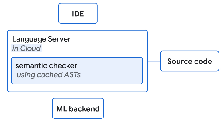


 NVIDIA Math Libraries are available to boost your application’s performance, from GPU-accelerated implementations of BLAS to random number generation.
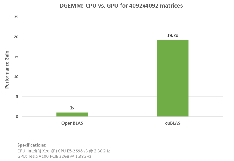
 How is speech AI related to AI, ML and DL? A quick guide on need-to-know speech AI terminologies like automatic speech recognition and text-to-speech.
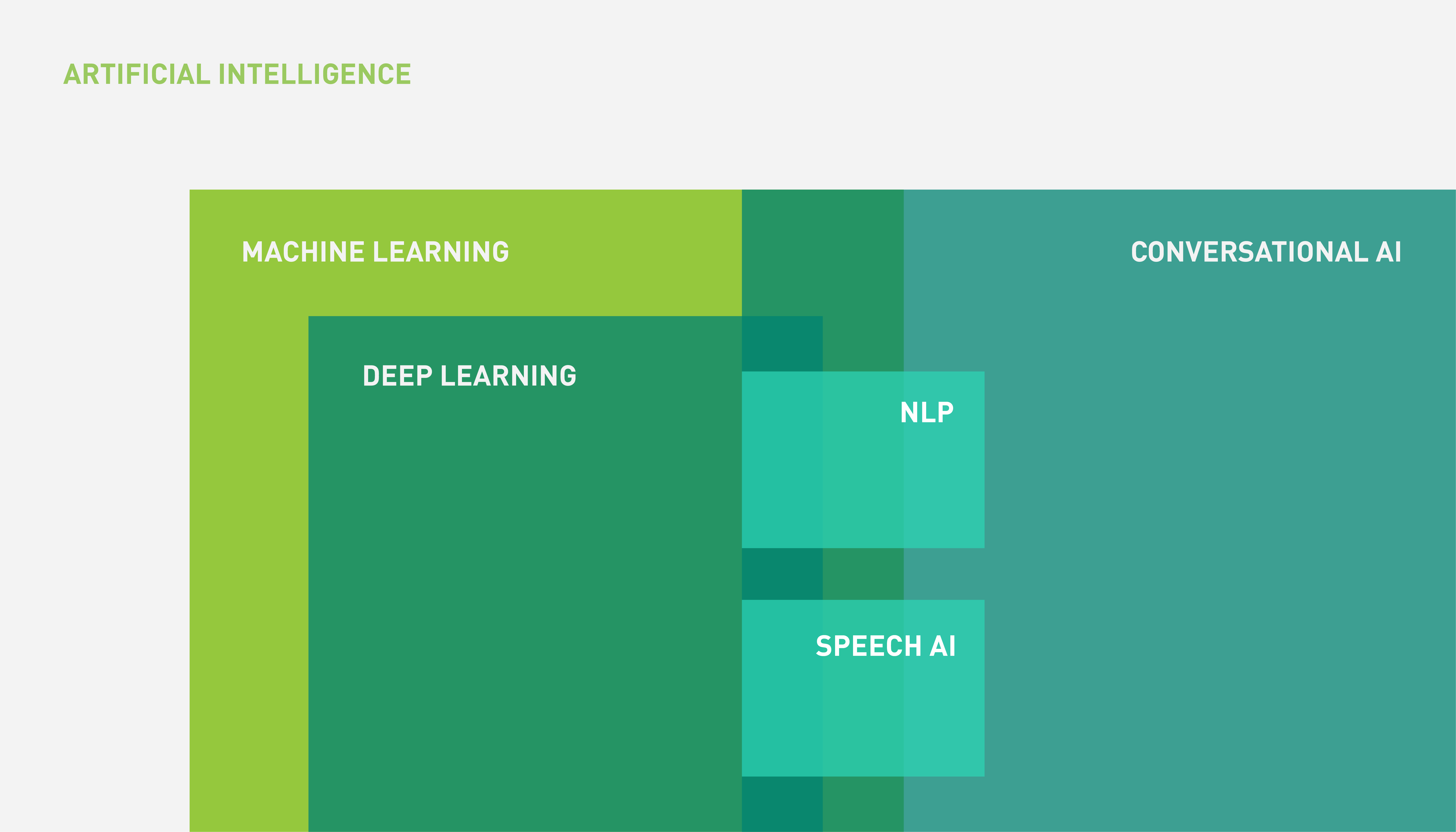
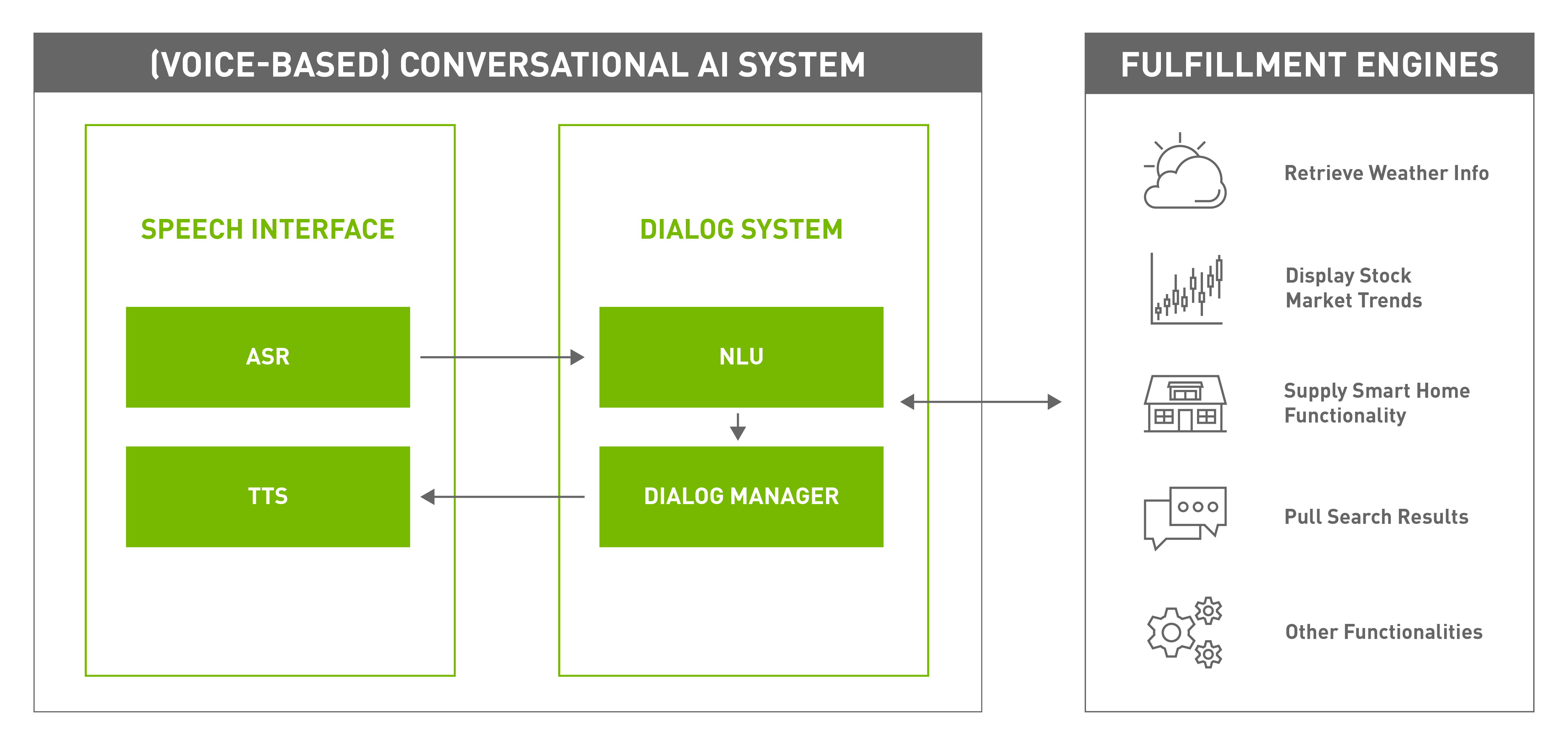
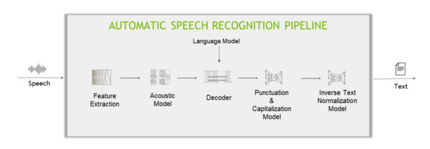
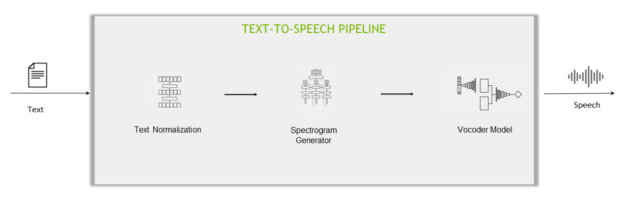
 Present barrier provides an easy way of synchronizing present calls between application windows on the same machine, as well as on distributed systems.
 NVIDIA Riva facilitates the process of creating ASR services with the tools and methodologies to help you realize your skills, all the way from raw data to a ready-to-use service.
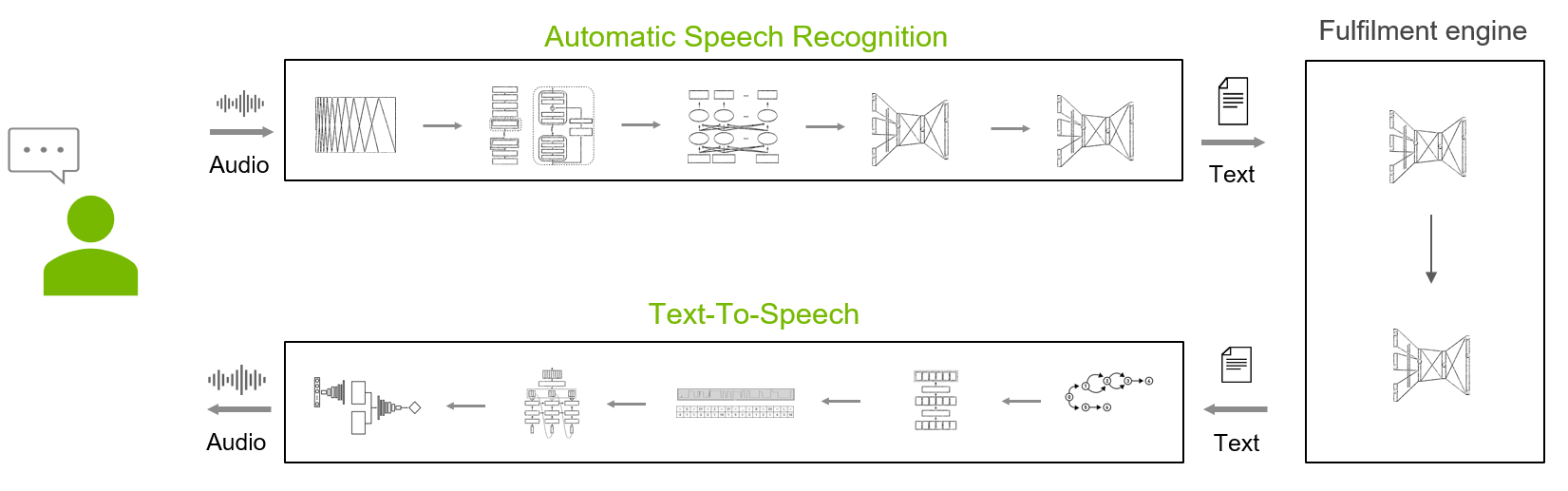
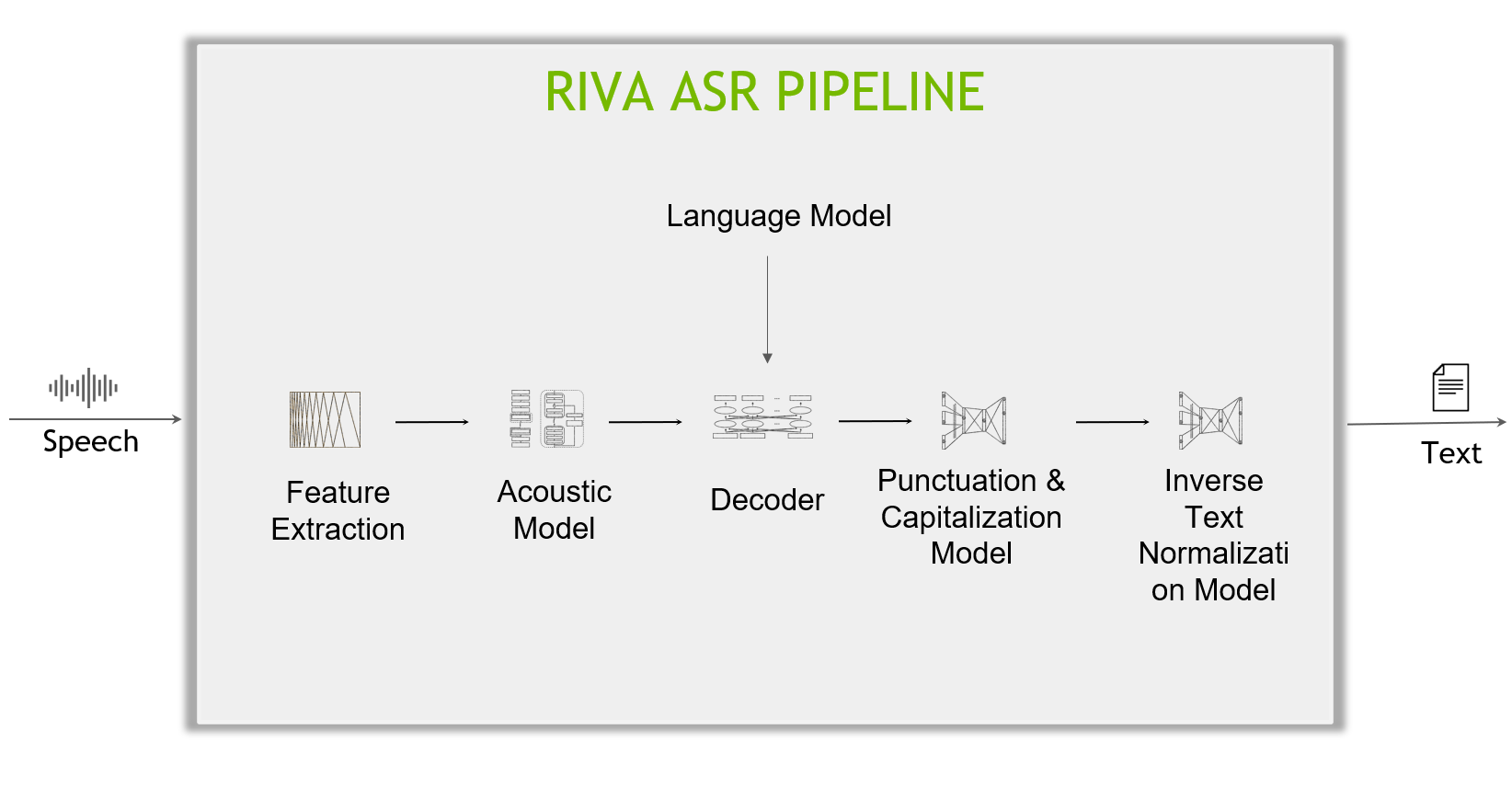
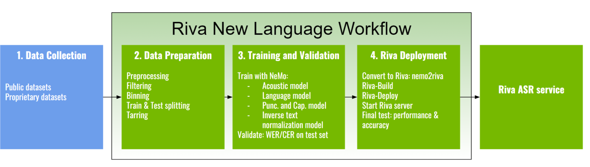

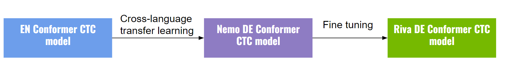
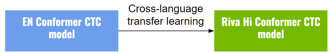
 Optimize your use of NVIDIA RTX with these in-depth ray tracing tips.
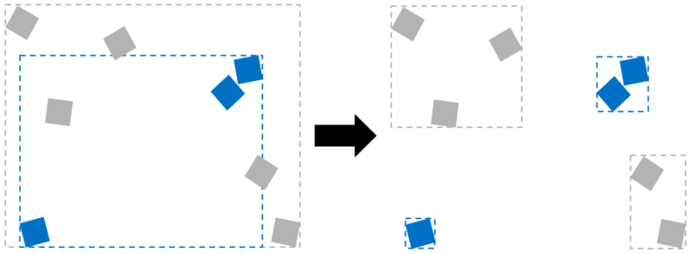
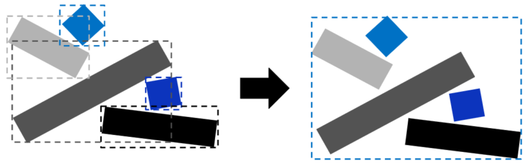
 Naive Bayes (NB) is a simple but powerful probabilistic classification technique that parallelizes well and can scale to datasets of massive size. If you have been working…