AttributeError: ‘google.protobuf.pyext._message.RepeatedCompositeCo’ object has no attribute ‘_values’
Protobuf version=3.15 Mediapiper version=0.8.6 Tensorflow version=2.5.0 I have tried installing all the version in virtual environment but error won’t go away.
This chapter, written by Juha Sjöholm, Paula Jukarainen, and Tatu Aalto, presents how all ray tracing based effects were implemented in Remedy Entertainment’s Control.
Next week, Ray Tracing Gems II will finally be available in its entirety as a free download, or for purchase as a physical release from Apress or Amazon. Since the start of July, we’ve been providing early access to a new chapter every week. Today’s chapter, by Juha Sjöholm, Paula Jukarainen, and Tatu Aalto, presents how all ray tracing based effects were implemented in Remedy Entertainment’s Control. This includes opaque and transparent reflections, near field indirect diffuse illumination, contact shadows, and the denoisers tailored for these effects.
You can also learn more about Game of the Year Winner Control here.
We’ve collaborated with our partners to make limited edition versions of the book, including custom covers that highlight real-time ray tracing in Fortnite, Control, and Watch Dogs: Legion.
NVIDIA GTC21 had numerous great and engaging contents, especially around RAPIDS, so it would be easy to miss our debut presentation “Using RAPIDS to Accelerate Node.js JavaScript for Visualization and Beyond.” Yep – we are bringing the power of GPU accelerated data science to the JavaScript Node.js community with the Node-RAPIDS project. Node-RAPIDS is an … Continued
Node-RAPIDS is an open-source, technical preview of modular RAPIDS’ library bindings in Node.js, as well as, complementary methods for enabling high-performance, browser-based visualizations.
What’s the problem with web viz?
Around a decade ago, the mini-renaissance around web-based data visualization showed the benefits of highly interactive, easy to share, and use tools such as D3. While not as performant as C/C++ or Python frameworks, their popularity took off because of JavaScript’s accessibility. No surprise that it often ranks as the most popular developer language, preceding Python or Java, and there is now a full catalog of visualization and data tools.
Yet, this large JavaScript community of developers is impeded by the lack of first-class and accelerated data tools in their preferred language. The analysis is most effective when it is paired as close as possible to its data source, science, and visualizations. To fully access GPU hardware with JavaScript, (beyond webGL limitations and hacks) requires being a polyglot to set up complicated middleware plumbing or use non-js frameworks like Plotly Dash. As a result, data engineers, data scientists, visualization specialists, and front-end developers are often siloed, even within organizations. This is detrimental because data visualization is the ideal medium of communication between these groups.
As for the RAPIDS Viz team, ever since our first proof of concept, we’ve wanted to build tools that can more seamlessly interact with hundreds of millions of data points in real-time through our browsers – and we finally have a way.
Why Node.js
If you are not familiar with Node.js, it is an open-source, cross-platform runtime environment based on C/C++ that executes JavaScript code outside of a web browser. Over 1 Million Node.js downloads occur perday. Node Package Manager (NPM) is the default JavaScript package manager and Microsoft owns it. Node.js is used in the backend of online marketplaces like eBay, AliExpress, and is used by high-traffic websites, such as Netflix, PayPal, and Groupon. Clearly, it is a powerful framework.
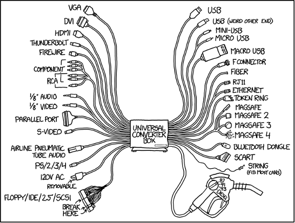
Figure 1: XKCD – Node.js is a Universal Connector.
Node.js is the connector that gives us JavaScript with direct access to hardware, which results in a streamlined API and the ability to use NVIDIA CUDA . By creating node-rapids bindings, we enable a massive developer community with the ability to use GPU acceleration without the need to learn a new language or work in a new environment. We also give the same community access to a high-performance data science platform: RAPIDS!
Here is a snippet of node-RAPIDS in action based on our basic notebook, which shows a 6x speedup for a small regex example:
Similar to node projects, Node-RAPIDS is designed to be modular. Our aim is not to build turnkey web applications, but to create an inventory of functionality that enables or accelerates a wide variety of use cases and pipelines. The preceding is an overview of the current and planned Node-RAPIDS modules grouped in general categories. A Node-RAPIDS application can use as many or as few of the modules as needed.
To make starting out less daunting, we are also building a catalog of demos that can serve as templates for generalized applications. As we develop more bindings, we will create more demos to showcase their capabilities.
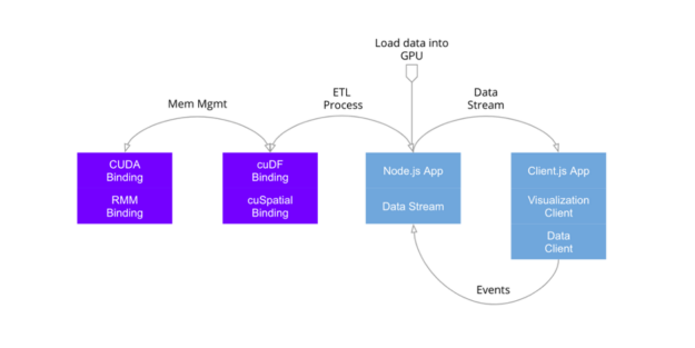
Figure 3: Example of a Cross Filter App.
The preceding is an idealized stack of a geospatial cross filter dashboard application using RAPIDS cuDF and RAPIDS cuSpatial libraries. We have a simple demo using Deck.gl that you can preview with our video and explore demo code on Github.
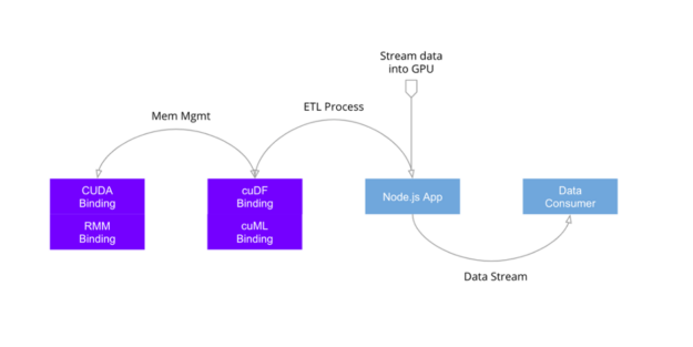
Figure 4: Example of Streaming ETL Process.
The last example preceding is a server-side only ETL pipeline without any visualization. We have an example of a straightforward ETL process using cuDF bindings and the nteract notebook desktop application, which you can preview with our video and nteract with (get it) on our Notebook.
What is next?
While we have been thinking about this project for a while, we are just getting started in development. RAPIDS is an incredible framework, and we want to bring it to more people and more applications – RAPIDS everywhere as we say.
Near-term next steps:
Some short-term next steps are to continue building core RAPIDS binding features, which you can check out on our current binding coverage table.
If the idea of GPU accelerated SQL queries straight from your web app sounds interesting (it does to us), we hope to get started on some blazingSQL bindings soon too.
And most noteworthy, we plan to start creating and publishing modular docker containers, which will dramatically simplify the current from-source tech preview installation process.
As always, we need community engagement to help guide us. If you have feature requests, questions, or use cases, you canreach out to us!
This project has numerous potentials. It can accelerate a wide variety of Node.js applications, as well as bring first-class, high-performance data science and visualization tools to a huge community. We hope you join us at the beginning of this exciting project.
Join the first NVIDIA Omniverse User Group, an exclusive event hosted by the lead engineers, designers, and artists of Omniverse on August 12, during the virtual SIGGRAPH conference.
Join the first NVIDIA Omniverse User Group, an exclusive event hosted by the lead engineers, designers, and artists of Omniverse on August 12, during the virtual SIGGRAPH conference.
The Omniverse User Group inaugural event is open to all developers, researchers, creators, students, professionals, and hobbyists of all levels, whether current Omniverse power users or curious explorers. The two-hour event will feature a look into the Omniverse roadmap, and provide sneak peeks of never-before-seen technologies and experiments.
Those who attend the Omniverse User Group will:
Hear the vision and future of Omniverse from Rev Lebaredian, VP of Omniverse & Simulation Technology, and Richard Kerris, VP of Omniverse Developer Platform
Learn how you can build on and extend the Omniverse ecosystem
Artists and developers can explore the latest news about NVIDIA Omniverse at SIGGRAPH. Watch the NVIDIA special address on Tuesday, August 10, at 8:00 am PDT to learn about the latest tools and solutions that are driving graphics, AI, and the emergence of shared worlds. The address will be presented by Richard Kerris, Vice President of Omniverse, and Sanja Fidler, Senior Director of AI Research at NVIDIA.
And tune in to the global premiere of “Connecting in the Metaverse: The Making of the GTC Keynote.” The new documentary premieres on August 11th at 9:00 am PDT, highlighting the creative minds and groundbreaking technologies behind the making of the NVIDIA GTC 2021 keynote. See how a small team of artists used NVIDIA Omniverse to blur the line between real and rendered.
Join NVIDIA at SIGGRAPH and learn more about the latest tools and technologies driving real-time graphics, AI-enhanced workflows and virtual collaboration.
There is a high chance that you have asked your smart speaker a question like, “How tall is Mount Everest?” If you did, it probably said, “Mount Everest is 29,032 feet above sea level.” Have you ever wondered how it found an answer for you? Question answering (QA) is loosely defined as a system consisting … Continued
There is a high chance that you have asked your smart speaker a question like, “How tall is Mount Everest?” If you did, it probably said, “Mount Everest is 29,032 feet above sea level.” Have you ever wondered how it found an answer for you?
Question answering (QA) is loosely defined as a system consisting of information retrieval (IR) and natural language processing (NLP), which is concerned with answering questions posed by humans in a natural language. If you are not familiar with information retrieval, it is a technique to obtain relevant information to a query, from a pool of resources, webpages, or documents in the database, for example. The easiest way to understand the concept is the search engine that you use daily.
You then need an NLP system to find an answer within the IR system that is relevant to the query. Although I just listed what you need for building a QA system, it is not a trivial task to build IR and NLP from scratch. Here’s how NVIDIA Riva makes it easy to develop a QA system.
Riva overview
NVIDIA Riva is an accelerated SDK for building multimodal conversational AI services that use an end-to-end deep learning pipeline. The Riva framework includes optimized services for speech, vision, and natural language understanding (NLU) tasks. In addition to providing several pretrained models for the entire pipeline of your conversational AI service, Riva is also architected for deployment at scale. In this post, I look closely into the QA function of Riva and how you can create your own QA application with it.
Riva QA function
To understand how the Riva QA function works, start with Bidirectional Encoder Representations from Transformers (BERT). It’s a transformer-based, NLP, pretraining method developed by Google in 2018, and it completely changed the field of NLP. BERT understands the contextual representation of a given word in a text. It is pretrained on a large corpus of data, including Wikipedia.
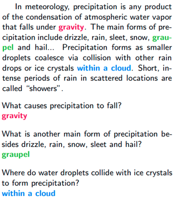
With the pretrained BERT, a strong NLP engine, you can further fine-tune it to perform QA with many question-answer pairs like those in the Stanford Question Answering Dataset (SQuAD). The model can now find an answer for a question in natural language from a given context: sentences or paragraphs. Figure 1 shows an example of QA, where it highlights the word “gravity” as an answer to the query, “What causes precipitation to fall?”. In this example, the paragraph is the context and the successfully fine-tuned QA model returns the word “gravity” as an answer.
Teams of engineers and researchers at NVIDIA deliver a quality QA function that you can use right out-of-the-box with Riva. The Riva NLP service provides a set of high-level API actions that include QA, NaturalQuery. TheWikipedia API action allows you to fetch articles posted on Wikipedia, an online encyclopedia, with a query in natural language. That’s the information retrieval system that I discussed earlier. Combining the Wikipedia API action and Riva QA function, you can create a simple QA system with a few lines of Python code.
Start by installing the Wikipedia API for Python. Next, import the Riva NLP service API and gRPC, the underlying communication framework for Riva.
!pip install wikipedia
import wikipedia as wiki
import grpc
import riva_api.riva_nlp_pb2 as rnlp
import riva_api.riva_nlp_pb2_grpc as rnlp_srv
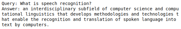
Now, create an input query. Use the Wikipedia API action to fetch the relevant articles and define the number of them to fetch, defined as max_articles_combine. Ask a question, “What is speech recognition?” You then print out the titles of the articles returned from the search. Finally, you add the summaries of each article into a variable: combined_summary.
input_query = "What is speech recognition?"
wiki_articles = wiki.search(input_query)
max_articles_combine = 3
combined_summary = ""
if len(wiki_articles) == 0:
    print("ERROR: Could not find any matching results in Wikipedia.")
else:
    for article in wiki_articles[:min(len(wiki_articles), max_articles_combine)]:
        print(f"Getting summary for: {article}")
        combined_summary += "n" + wiki.summary(article)
Figure 2. Titles of articles fetched by Wikipedia API action.
Next, open a gRPC channel that points to the location where the Riva server is running. Because you are running the Riva server locally, it is ‘localhost:50051‘. Then, instantiate NaturalQueryRequest, and send a request to the Riva server, passing both the query and the context. Finally, print the response, returned from the Riva server.
With Riva QA and the Wikipedia API action, you just created a simple QA application. If there’s an article in Wikipedia that is relevant to your query, you can theoretically find answers. Imagine that you have a database full of articles relevant to your domain, company, industry, or anything of interest. You can create a QA service that can find answers to the questions specific to your field of interest. Obviously, you would need an IR system that would fetch relevant articles from your database, like the Wikipedia API action used in this post. When you have the IR system in your pipeline, Riva can help you find an answer for you. We look forward to the cool applications that you’ll create with Riva. .
9 Down, 14 letters: Someone skilled in creating and solving crossword puzzles. This April, the fastest “cruciverbalist” at the American Crossword Puzzle Tournament was Dr.Fill, a crossword puzzle-solving AI program created by Matt Ginsberg. Dr.Fill perfectly solved the championship puzzle in 49 seconds. The first human champion, Tyler Hinman, filled the 15×15 crossword in exactly Read article >
NVIDIA announces the newest release of the CUDA development environment, CUDA 11.4. This release includes GPU-accelerated libraries, debugging and optimization tools, programming language enhancements, and a runtime library to build and deploy your application on GPUs across the major CPU architectures: x86, Arm, and POWER. CUDA 11.4 is focused on enhancing the programming model and … Continued
NVIDIA announces the newest release of the CUDA development environment, CUDA 11.4. This release includes GPU-accelerated libraries, debugging and optimization tools, programming language enhancements, and a runtime library to build and deploy your application on GPUs across the major CPU architectures: x86, Arm, and POWER.
CUDA 11.4 is focused on enhancing the programming model and performance of your CUDA applications. CUDA continues to push the boundaries of GPU acceleration and lay the foundation for new applications in HPC, graphics, CAE applications, AI and deep learning, automotive, healthcare, and data sciences.
CUDA 11.4 has several important features. This post offers an overview of the key capabilities:
CUDA Programming model enhancements:
CUDA Graphs
Multi-Process Service (MPS)
Formalizing Asynchronous Data Movement
C++ Language support – CUDA
Compiler enhancements
CUDA Driver Enhancements
CUDA 11.4 ships with the R470 driver, which is a long-term support branch. GPUDirect RDMA and GPUDirect technology Storage (GDS) are now part of the CUDA Driver and Toolkit. This streamlines the workflow and enables our developers to leverage these technologies without the need for separate installation of additional packages. The driver enables new MIG configurations for the recently launched NVIDIA A30 GPU, which doubles the memory per MIG slice. This results in greater peak performance for various workloads on the A30 GPU, especially for AI inference workloads.
This release introduced key enhancements to improve the performance of CUDA Graphs without requiring any modifications to the application or any other user intervention. It also improves the ease of use of Multi-Process Service (MPS). We formalized the asynchronous programming model in the CUDA Programming Guide.
CUDA Graphs
Reducing graph launch latency is a common request from the developer community, especially in applications that have real-time constraints, such as 5G telecom workloads or AI inference workloads. CUDA 11.4 delivers performance improvements in reducing the CUDA graph launch times. In addition, we also integrated the stream-ordered memory allocation feature that was introduced in CUDA 11.2.
CUDA graphs are ideal for workloads that are executed multiple times, so a key tradeoff in choosing graphs for a workload is amortizing the cost of creating a graph over repeated launches. The higher the number of repetitions or iterations, the larger the performance improvement.
In CUDA 11.4, we made a couple of key changes to CUDA graph internals that further improve the launch performance. CUDA graphs already sidesteps streams to enable lower latency runtime execution. We extended this, to bypass streams even at the launch phase, submitting a graph as a single block of work directly to the hardware. We’ve seen good performance gains from these host improvements, both for single-threaded and multithreaded applications.
Figure 1 shows the relative improvement in launch latency for the re-launch of different graph patterns. There is significant benefit for graphs that have a fork or join pattern.
Figure 1.Launch latency performance improvement for a single graph for repeat launches with CUDA 11.3 baselines.
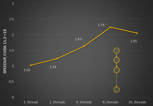
Multithreaded launch performance is particularly affected by the resource contention that happens when launching multiple graphs in parallel. We’ve optimized the interthread locking to reduce contention, and so multithreaded launch is now significantly more efficient. Figure 2 shows the relative performance benefits of the changes in CUDA 11.4 to ease resource contention and how it scales with the number of threads.
Figure 2.Multithreaded launch latency improvement for a straight line for repeat launches with CUDA 11.3 baselines.
Stream-ordered memory allocator support
The stream-ordered memory allocator enables applications to order memory allocation and deallocation with respect to other work launched into a CUDA stream. This also enables allocation re-use, which can significantly improve application performance. For more information about the feature and capabilities, see Enhancing Memory Allocation with New NVIDIA CUDA 11.2 Features.
In CUDA 11.4, CUDA Graphs now supports stream-ordered memory allocation both through stream capture or in native graph construction through new allocate and free node types, enabling the same efficient, deferred memory reuse logic within graphs.
These node types are collectively referred to as memory nodes. They can be created in several ways:
Using the explicit API
Using cudaGraphAddMemAllocNode and cudaGraphAddMemFreeNode, respectively
Using stream capture
Using cudaMallocAsync/cudaMallocFromPoolAsync and cudaFreeAsync, respectively
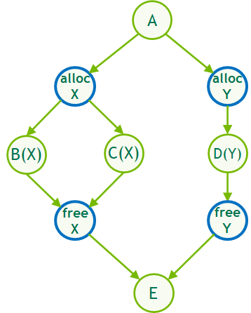
In the same way that stream-ordered allocation uses implicit stream ordering and event dependencies to reuse memory, graph-ordered allocation uses the dependency information defined by the edges of the graph to do the same.
Figure 3. Intra-graph memory reuse. When a MemAlloc node is created, it attempts to reuse memory, which was freed by MemFree nodes that it depends upon.
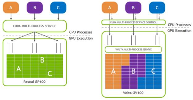
The Multi-Process Service (MPS) is a binary-compatible client-server runtime implementation of the CUDA API designed to transparently enable co-operative multiprocess CUDA applications.
It consists of a control daemon process, client runtime, and server process. MPS enables better GPU utilization in cases where a single process does not use all the compute and memory-bandwidth capacity. MPS also reduces on-GPU context storage and context switching. For more information, see Multi-Process Service in the GPU Management and Deployment guide.
In this release, we made a couple of key enhancements to improve the ease of use of MPS.
Figure 4.Schematic representation of MPS with reduced on-GPU context storage and context switching to improve ease-of-use.
Programmatic configuration of SM partitions
There are certain use cases that share the following characteristics:
They consist of kernels that have little to no interaction, which enables concurrent execution.
The ratio of SMs required by these workloads may change and requires flexibility in allocating the right number of SMs.
The MPS active thread percentage setting enables you to limit the execution to a portion of the SMs. Before CUDA 11.4, this was a fixed value that was set equally for all clients within the process. In CUDA 11.4, this has been extended to offer a mechanism to partition the SMs at a per-client level through a programmatic interface. This enables you to create contexts that have different SM partitions within the same application process.
A new resource type called CU_EXEC_AFFINITY_TYPE_SM_COUNT enables you to specify a minimum number N that the context requires. The system guarantees that at least this many SMs are assigned, although more may be reserved. CUDA 11.4 also introduces a related affinity API cuCtxGetExecAffinity, which queries the exact amount of a resource (such as the SM count) allocated for a context. For more information, see the cuCtxGetExecAffinity section in the API documentation.
Error reporting
To improve the error reporting and ease of diagnosing the root cause of MPS issues, we introduced new and detailed driver and runtime error codes. These error codes provide more specificity regarding the type of error. They supplement the common MPS error codes with additional information to help you trace down the cause of the failures. Use these error codes in your applications with the error messages in the server log, as part of the root cause analysis.
In support of the asynchronous memory transfer operations, enabled by NVIDIA A100 GPU microarchitecture, in CUDA 11.4, we formalized and defined the asynchronous SIMT programming model. The asynchronous programming model defines the behavior and the APIs for C++ 20 barriers and cuda::memcpy_async on the GPU.
For more information about how you can use the asynchronous APIs to overlap memory operations from global memory, with computations in the streaming multiprocessors (SMs), see Asynchronous SIMT Programming Model.
Other enhancements
In addition to the key capabilities listed earlier, there are a few enhancements in CUDA 11.4 geared towards improving the mulit-thread submission throughput and extending the CUDA forward compatibility support to NVIDIA RTX GPUs.
Multithread submission throughput
In 11.4, we reduced the serialization of the CUDA API overheads between CPU threads. These changes are enabled by default. However, to assist with the triage of possible issues because of the underlying changes, we provide an environment variable, CUDA_REDUCE_API_SERIALIZATION, to turn off these changes. This was one of the underlying changes discussed earlier that contributed to the performance improvements for CUDA graphs.
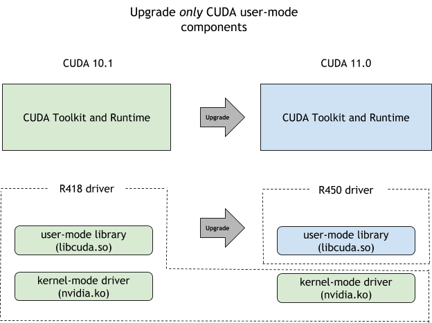
CUDA forward compatibility
To enable use cases where you want to update your CUDA toolkit but stay on your current driver version, for example to reduce the risk or the overhead of additional validation needed to move to a new driver, CUDA offers the CUDA forward compatibility path. This was introduced in CUDA 10.0 but was initially limited to data-center GPUs. CUDA 11.4 eases those restrictions and you can now take advantage of the forward compatibility path for NVIDIA RTX GPUs as well.
Figure 5.Forward compatibility upgrade path between pre-CUDA 11.0 releases and current CUDA 11.x drivers.
C++ language support for CUDA
Here are some key enhancements included with C++ language support in CUDA 11.4.
Major releases:
NVIDIA C++ Standard Library (libcu++) 1.5.0 was released with CUDA 11.4.
Thrust 1.12.0 has the new thrust::universal_vector API that enables you to use the CUDA unified memory with Thrust.
Bug fix release: The CUDA 11.4 toolkit release includes CUB 1.12.0.
New asynchronous thrust::async:exclusive_scan and inclusive_scan algorithms have been added, and the synchronous versions of these were updated to use cub::DeviceScan directly.
CUDA compiler enhancements
CUDA 11.4 NVCC C++ compiler has JIT LTO support in preview, offers more L1 and L2 cache control, and exposes a C++ symbol demangling static library along with NVIDIA Nsight debugger support for alloca.
JIT link time optimization
JIT link-time optimization (LTO) is a preview feature and is available only on CUDA Toolkit 11.4, not on embedded platforms. This feature enables LTO to be performed at runtime. Use NVRTC to generate NVVM IR, and then use the cuLink driver APIs to link the NVVM IR and do LTO.
The following code example shows how runtime JIT LTO can be used in your program. Generate NVVM IR using nvrtcCompileProgram with the -dlto option and retrieve the generated NVVM IR using the newly introduced nvrtcGetNVVM. Existing cuLink APIs are augmented to take newly introduced JIT LTO options to accept NVVM IR as input and to perform JIT LTO. Pass the CU_JIT_LTO option to cuLinkCreate API to instantiate the linker and then use CU_JIT_INPUT_NVVM as option to cuLinkAddFile or cuLinkAddData API for further linking of NVVM IR.
The CUDA SDK now ships with libcu++filt, a static library that converts compiler-mangled C++ symbols into user-readable names. The following API, found in the nv_decode.h header file, is the entry point to the library:
char* __cu_demangle(const char* id, char *output_buffer, size_t *length, int *status)
The following C++ example code shows usage:
 #include
 #include "/usr/local/cuda-14.0/bin/nv_decode.h"

 using namespace std;
 int main(int argc, char **argv)
 {
   const char* mangled_name = "_ZN6Scope15Func1Enez";
   int status = 1;
   char* w = __cu_demangle(mangled_name,0,0,&status);
   if(status != 0)
     cout


This code example outputs as follows:


Demangling Succeeded: Scope1::Func1(__int128, long double, ...)
Demangling Succeeded: Scope1::Func1(__int128, long double, ...)
For more information, see Library Availability in the CUDA Binary Utilities documentation.
Configuring cache behavior in PTX
PTX ISA 7.4 gives you more control over caching behavior of both L1 and L2 caches. The following capabilities are introduced in this PTX ISA version:
Enhanced data prefetching: The new .level::prefetch_size qualifier can be used to prefetch additional data along with memory load or store operations. This enables exploiting the spatial locality of data.
Eviction priority control: PTX ISA 7.4 introduces four cache eviction priorities. These eviction priorities can be specified with the .level::eviction_priority qualifier on memory load or store operations (applicable to the L1 cache) and on the prefetch instruction (applicable to the L2 cache).
evict_normal (default)
evict_last (useful when the data should be kept in the cache longer)
evict_first (useful for streaming data)
no_allocate (avoid data from being cached at all)
Enhanced L2 cache control: This comes in two flavors:
Cache control on specific addresses: The new discard instruction enables discarding data from cache without writing it back to memory. It should be only used when the data is no longer required. The new applypriority instruction sets the eviction priority of specific data to evict_normal. This is [articularly useful in downgrading the eviction priority from evict_last when the data no longer needs to be persistent in cache.
Cache-hints on memory operations: The new createpolicy instruction enables creating a cache policy descriptor that encodes one or more cache eviction priorities for different data regions. Several memory operations including load, store, asynchronous copy, atom, red, and so on can accept cache policy descriptor as an operand when the .level::cache_hint qualifier is used.
These extensions are treated as performance hints only. The caching behavior specified using these extensions is not guaranteed by the caching system. For more information about usage, see the PTX ISA specification.
Other compiler enhancements in CUDA 11.4 include support for a new host compiler: ICC 2021. The diagnostics emitted by the CUDA frontend compiler are now ANSI colored and Nsight debugger can now correctly unwind CUDA applications with alloca calls, in the Call Stack view.
Nsight Developer Tools
New versions are now available for NVIDIA Nsight Visual Studio Code Edition (VSCE) and Nsight Compute 2021.2, adding enhancements to the developer experience for CUDA programming.
NVIDIA Nsight VSCE is an application development environment for heterogeneous platforms bringing CUDA development for GPUs into Microsoft Visual Studio Code. NVIDIA Nsight VSCE enables you to build and debug GPU kernels and native CPU code in the same session as well as inspect the state of the GPU and memory.
It includes IntelliSense code highlighting for CUDA applications and an integrated GPU debugging experience from the IDE with support for stepping through code, setting breakpoint, and inspecting memory states and system information in CUDA kernels. Now it’s easy to develop and debug CUDA applications directly from Visual Studio Code.
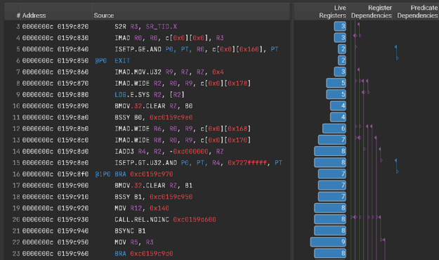
Nsight Compute 2021.2 adds new features that help detect more performance issues and make it easier to understand and fix them. The new register dependency visualization (Figure 6) helps identify long dependency chains and inefficient register usage that can limit performance. This release also adds a frequently requested feature to enable you to view the side-by-side assembly and correlated source code for CUDA kernels in the source view, without needing to collect a profile. This standalone source viewer feature enables you to open .cubin files directly from disk in the GUI to see the code correlation.
Figure 6. Nsight Compute Register Dependency Visualization capability helps identify long dependency chains and inefficient register usage to help improve performance.
Several features, including highlighted focus metrics, report cross-links, increased rule visibility, and documentation references all add to the built-in profile and optimization guided analysis that Nsight Compute provides to help you understand and fix performance bottlenecks.
This release also includes support for OptiX 7 resource tracking, a new Python interface for reading report data, and improvements to management of baseline reports, font settings, and CLI filters.
Most CUDA developers are familiar with the cudaMalloc and cudaFree API functions to allocate GPU accessible memory. However, there has long been an obstacle with these API functions: they aren’t stream ordered. In this post, we introduce new API functions, cudaMallocAsync and cudaFreeAsync, that enable memory allocation and deallocation to be stream-ordered operations. In part … Continued
Most CUDA developers are familiar with the cudaMalloc and cudaFree API functions to allocate GPU accessible memory. However, there has long been an obstacle with these API functions: they aren’t stream ordered. In this post, we introduce new API functions, cudaMallocAsync and cudaFreeAsync, that enable memory allocation and deallocation to be stream-ordered operations.
In part 2 of this series, we highlight the benefits of this new capability by sharing some big data benchmark results and provide a code migration guide for modifying your existing applications. We also cover advanced topics to take advantage of stream-ordered memory allocation in the context of multi-GPU access and the use of IPC. This all helps you improve performance within your existing applications.
Stream ordering efficiency
The following code example on the left is inefficient because the first cudaFree call has to wait for kernelA to finish, so it synchronizes the device before freeing the memory. To make this run more efficiently, the memory can be allocated upfront and sized to the larger of the two sizes, as shown on the right.
cudaMalloc(&ptrA, sizeA);
kernelA>>(ptrA);
cudaFree(ptrA); // Synchronizes the
device before freeing memory
cudaMalloc(&ptrB, sizeB);
kernelB>>(ptrB);
cudaFree(ptrB);
This increases code complexity in the application because the memory management code is separated out from the business logic. The problem is exacerbated when other libraries are involved. For example, consider the case where kernelA is launched by a library function instead:
This is much harder for the application to make efficient because it may not have complete visibility or control over what the library is doing. To circumvent this problem, the library would have to allocate memory when that function is invoked for the first time and never free it until the library is deinitialized. This not only increases code complexity, but it also causes the library to hold on to the memory longer than it needs to, potentially denying another portion of the application from using that memory.
Some applications take the idea of allocating memory upfront even further by implementing their own custom allocator. This adds a significant amount of complexity to application development. CUDA aims to provide a low-effort, high-performance alternative.
CUDA 11.2 introduced a stream-ordered memory allocator to solve these types of problems, with the addition of cudaMallocAsync and cudaFreeAsync. These new API functions shift memory allocation from global-scope operations that synchronize the entire device to stream-ordered operations that enable you to compose memory management with GPU work submission. This eliminates the need for synchronizing outstanding GPU work and helps restrict the lifetime of the allocation to the GPU work that accesses it. Consider the following code example:
cudaMallocAsync(&ptrA, sizeA, stream);
kernelA>>(ptrA);
cudaFreeAsync(ptrA, stream); // No synchronization necessary
cudaMallocAsync(&ptrB, sizeB, stream); // Can reuse the memory freed previously
kernelB>>(ptrB);
cudaFreeAsync(ptrB, stream);
It is now possible to manage memory at function scope, as in the following example of a library function launching kernelA.
libraryFuncA(stream);
cudaMallocAsync(&ptrB, sizeB, stream); // Can reuse the memory freed by the library call
kernelB>>(ptrB);
cudaFreeAsync(ptrB, stream);

void libraryFuncA(cudaStream_t stream) {
    cudaMallocAsync(&ptrA, sizeA, stream);
    kernelA>>(ptrA);
    cudaFreeAsync(ptrA, stream); // No synchronization necessary
}
Stream-ordered allocation semantics
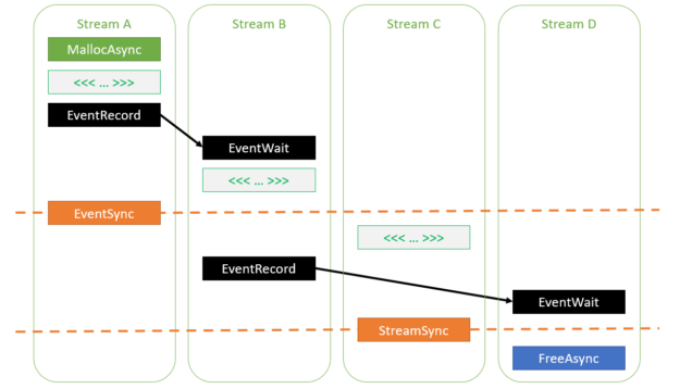
All the usual stream-ordering rules apply to cudaMallocAsync and cudaFreeAsync. The memory returned from cudaMallocAsync can be accessed by any kernel or memcpy operation as long as the kernel or memcpy is ordered to execute after the allocation operation and before the deallocation operation, in stream order. Deallocation can be performed in any stream, as long as it is ordered to execute after the allocation operation and after all accesses on all streams of that memory on the GPU.
In effect, stream-ordered allocation behaves as if allocation and free were kernels. If kernelA produces a valid buffer on a stream and kernelB invalidates it on the same stream, then an application is free to access the buffer after kernelA and before kernelB in the appropriate stream order.
The following example shows various valid usages.
auto err = cudaMallocAsync(&ptr, size, streamA);
// If cudaMallocAsync completes successfully, ptr is guaranteed to be
// a valid pointer to memory that can be accessed in stream order

assert(err == cudaSuccess);

// Work launched in the same stream can access the memory because
// operations within a stream are serialized by definition

kernel>>(ptr);

// Work launched in another stream can access the memory as long as
// the appropriate dependencies are added

cudaEventRecord(event, streamA);
cudaStreamWaitEvent(streamB, event, 0);
kernel>>(ptr);


// Synchronizing the stream at a point beyond the allocation operation
// also enables any stream to access the memory

cudaEventSynchronize(event);
kernel>>(ptr);

// Deallocation requires joining all the accessing streams. Here,
// streamD will be deallocating.
// Adding an event dependency on streamB ensures that all accesses in
// streamB will be done before the deallocation

cudaEventRecord(event, streamB);
cudaStreamWaitEvent(streamD, event, 0);

// Synchronizing streamC also ensures that all its accesses are done before
// the deallocation

cudaStreamSynchronize(streamC);
cudaFreeAsync(ptr, streamD);
Figure 1 shows the various dependencies specified in the earlier code example. As you can see, all kernels are ordered to execute after the allocation operation and complete before the deallocation operation.
Figure 1. Various ways to insert dependencies between streams to ensure correctness when accessing memory allocated using cudaMallocAsync.
Memory allocation and deallocation cannot fail asynchronously. Memory errors that occur because of a call to cudaMallocAsync or cudaFreeAsync (for example, out of memory) are reported immediately through an error code returned from the call. If cudaMallocAsync completes successfully, the returned pointer is guaranteed to be a valid pointer to memory that is safe to access in the appropriate stream order.
err = cudaMallocAsync(&ptr, size, stream);
if (err != cudaSuccess) {
    return err;
}
// Now you’re guaranteed that ‘ptr’ is valid when the kernel executes on stream
kernel>>(ptr);
cudaFreeAsync(ptr, stream);
The CUDA driver uses memory pools to achieve the behavior of returning a pointer immediately.
Memory pools
The stream-ordered memory allocator introduces the concept of memory pools to CUDA. A memory pool is a collection of previously allocated memory that can be reused for future allocations. In CUDA, a pool is represented by a cudaMemPool_t handle. Each device has a notion of a default pool whose handle can be queried using cudaDeviceGetDefaultMemPool.
You can also explicitly create your own pools and either use them directly or set them as the current pool for a device and use them indirectly. Reasons for explicit pool creation include custom configuration, as described later in this post. When no explicitly created pool has been set as the current pool for a device, the default pool acts as the current pool.
When called without an explicit pool argument, each call to cudaMallocAsync infers the device from the specified stream and attempts to allocate memory from that device’s current pool. If the pool has insufficient memory, the CUDA driver calls into the OS to allocate more memory. Each call to cudaFreeAsync returns memory to the pool, which is then available for re-use on subsequent cudaMallocAsync requests. Pools are managed by the CUDA driver, which means that applications can enable pool sharing between multiple libraries without those libraries having to coordinate with each other.
If a memory allocation request made using cudaMallocAsync can’t be serviced due to fragmentation of the corresponding memory pool, the CUDA driver defragments the pool by remapping unused memory in the pool to a contiguous portion of the GPU’s virtual address space. Remapping existing pool memory instead of allocating new memory from the OS also helps keep the application’s memory footprint low.
By default, unused memory accumulated in the pool is returned to the OS during the next synchronization operation on an event, stream, or device, as the following code example shows.
cudaMallocAsync(ptr1, size1, stream); // Allocates new memory into the pool
kernel>>(ptr);
cudaFreeAsync(ptr1, stream); // Frees memory back to the pool
cudaMallocAsync(ptr2, size2, stream); // Allocates existing memory from the pool
kernel>>(ptr2);
cudaFreeAsync(ptr2, stream); // Frees memory back to the pool
cudaDeviceSynchronize(); // Frees unused memory accumulated in the pool back to the OS
// Note: cudaStreamSynchronize(stream) achieves the same effect here
Retaining memory in the pool
Returning memory from the pool to the system can affect performance in some cases. Consider the following code example:
for (int i = 0; i >>(ptr);
    cudaFreeAsync(ptr, stream);
    cudaStreamSynchronize(stream);
}
By default, stream synchronization causes any pools associated with that stream’s device to release all unused memory back to the system. In this example, that would happen at the end of every iteration. As a result, there is no memory to reuse for the next cudaMallocAsync call and instead memory must be allocated through an expensive system call.
To avoid this expensive reallocation, the application can configure a release threshold to enable unused memory to persist beyond the synchronization operation. The release threshold specifies the maximum amount of memory the pool caches. It releases all excess memory back to the OS during a synchronization operation.
By default, the release threshold of a pool is zero. This means that allunused memory in the pool is released back to the OS during every synchronization operation. The following code example shows how to change the release threshold.
cudaMemPool_t mempool;
cudaDeviceGetDefaultMemPool(&mempool, device);
uint64_t threshold = UINT64_MAX;
cudaMemPoolSetAttribute(mempool, cudaMemPoolAttrReleaseThreshold, &threshold);
for (int i = 0; i >>(ptr);
    cudaFreeAsync(ptr, stream);
    cudaStreamSynchronize(stream);    // Only releases memory down to “threshold” bytes
}
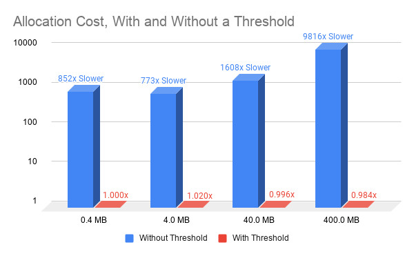
Using a nonzero release threshold enables reusing memory from one iteration to the next. This requires only simple bookkeeping and makes the performance of cudaMallocAsync independent of the size of the allocation, which results in dramatically improved memory allocation performance (Figure 2).
Figure 2. Cost of allocating memory using cudaMallocAsync with and without setting a release threshold (all values relative to performance of 0.4MB with threshold allocation).
The pool threshold is just a hint. Memory in the pool can also be released implicitly by the CUDA driver to enable an unrelated memory allocation request in the same process to succeed. For example, a call to cudaMalloc or cuMemCreate could cause CUDA to free unused memory from any memory pool associated with the device in the same process to serve the request.
This is especially helpful in scenarios where an application makes use of multiple libraries, some of which use cudaMallocAsync and some that do not. By automatically freeing up unused pool memory, those libraries do not have to coordinate with each other to have their respective allocation requests succeed.
There are limitations to when the CUDA driver automatically reassigns memory from a pool to unrelated allocation requests. For example, the application may be using a different interface, like Vulkan or DirectX, to access the GPU, or there may be more than one process using the GPU at the same time. Memory allocation requests in those contexts do not cause automatic freeing of unused pool memory. In such cases, the application may have to explicitly free unused memory in the pool, by invoking cudaMemPoolTrimTo.
The bytesToKeep argument tells the CUDA driver how many bytes it can retain in the pool. Any unused memory that exceeds that size is released back to the OS.
Better performance through memory reuse
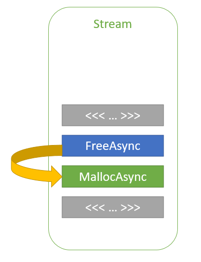
The stream parameter to cudaMallocAsync and cudaFreeAsync helps CUDA reuse memory efficiently and avoid expensive calls into the OS. Consider the following trivial code example.
In this code example, ptr2 is allocated in stream order after ptr1 is freed. The ptr2 allocation could reuse some, or all, of the memory that was used for ptr1 without any synchronization, because kernelA and kernelB are launched in the same stream. So, stream-ordering semantics guarantee that kernelB cannot begin execution and access the memory until kernelA has completed. This way, the CUDA driver can help keep the memory footprint of the application low while also improving allocation performance.
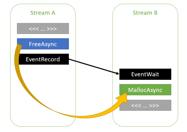
The CUDA driver can also follow dependencies between streams inserted through CUDA events, as shown in the following code example:
Figure 4. Memory reuse across streams with an event dependency between them.
As the CUDA driver is aware of the dependency between streams A and B, it can reuse the memory used by ptr1 for ptr2. The dependency chain between streams A and B can contain any number of streams, as shown in the following code example.
cudaMallocAsync(&ptr1, size1, streamA);
kernelA>>(ptr1);
cudaFreeAsync(ptr1, streamA);
cudaEventRecord(event, streamA);
for (int i = 0; i >>(ptr2);
If necessary, the application can disable this feature on a per-pool basis:
int enable = 0;
cudaMemPoolSetAttribute(mempool, cudaMemPoolReuseFollowEventDependencies, &enable);
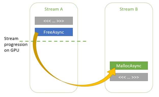
The CUDA driver can also reuse memory opportunistically in the absence of explicit dependencies specified by the application. While such heuristics may help improve performance or avoid memory allocation failures, they can add nondeterminism to the application and so can be disabled on a per-pool basis. Consider the following code example:
In this scenario, there are no explicit dependencies between streamA and streamB. However, the CUDA driver is aware of how far each stream has executed. If, on the second call to cudaMallocAsync in streamB, the CUDA driver determines that kernelA has finished execution on the GPU, then it can reuse some or all of the memory used by ptr1 for ptr2.
Figure 5. Opportunistic memory reuse across streams.
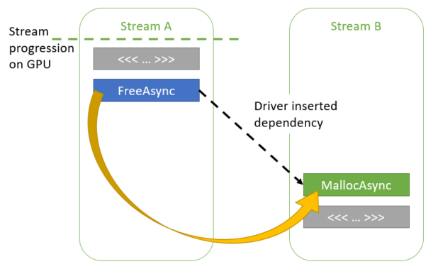
If kernelA has not finished execution, the CUDA driver can add an implicit dependency between the two streams such that kernelB does not begin executing until kernelA finishes.
Figure 6. Memory reuse through internal dependencies.
The application can disable these heuristics as follows:
int enable = 0;
cudaMemPoolSetAttribute(mempool, cudaMemPoolReuseAllowOpportunistic, &enable);
cudaMemPoolSetAttribute(mempool, cudaMemPoolReuseAllowInternalDependencies, &enable);
Summary
In part 1 of this series, we introduced the new API functions cudaMallocAsync and cudaFreeAsync , which enable memory allocation and deallocation to be stream-ordered operations. Use them to avoid expensive calls to the OS through memory pools maintained by the CUDA driver.
In part 2 of this series, we share some benchmark results to show the benefits of stream-ordered memory allocation. We also provide a step-by-step recipe for modifying your existing applications to take full advantage of this advanced CUDA capability.

 This chapter, written by Juha Sjöholm, Paula Jukarainen, and Tatu Aalto, presents how all ray tracing based effects were implemented in Remedy Entertainment’s Control.
 NVIDIA GTC21 had numerous great and engaging contents, especially around RAPIDS, so it would be easy to miss our debut presentation “Using RAPIDS to Accelerate Node.js JavaScript for Visualization and Beyond.” Yep – we are bringing the power of GPU accelerated data science to the JavaScript Node.js community with the Node-RAPIDS project. Node-RAPIDS is an …
 . By creating node-rapids bindings, we enable a massive developer community with the ability to use GPU acceleration without the need to learn a new language or work in a new environment. We also give the same community access to a high-performance data science platform: RAPIDS!
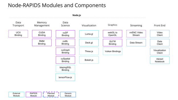
 Join the first NVIDIA Omniverse User Group, an exclusive event hosted by the lead engineers, designers, and artists of Omniverse on August 12, during the virtual SIGGRAPH conference.
 There is a high chance that you have asked your smart speaker a question like, “How tall is Mount Everest?” If you did, it probably said, “Mount Everest is 29,032 feet above sea level.” Have you ever wondered how it found an answer for you? Question answering (QA) is loosely defined as a system consisting …


 NVIDIA announces the newest release of the CUDA development environment, CUDA 11.4. This release includes GPU-accelerated libraries, debugging and optimization tools, programming language enhancements, and a runtime library to build and deploy your application on GPUs across the major CPU architectures: x86, Arm, and POWER. CUDA 11.4 is focused on enhancing the programming model and …
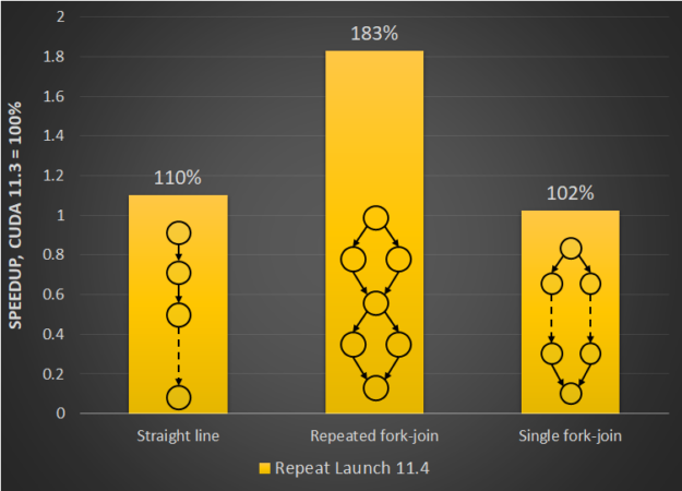
 Most CUDA developers are familiar with the cudaMalloc and cudaFree API functions to allocate GPU accessible memory. However, there has long been an obstacle with these API functions: they aren’t stream ordered. In this post, we introduce new API functions, cudaMallocAsync and cudaFreeAsync, that enable memory allocation and deallocation to be stream-ordered operations. In part …