Crafted by AI for AI, GPUNet is a class of convolutional neural networks designed to maximize the performance of NVIDIA GPUs using NVIDIA TensorRT. Built using…
Crafted by AI for AI, GPUNet is a class of convolutional neural networks designed to maximize the performance of NVIDIA GPUs using NVIDIA TensorRT.
Built using novel neural architecture search (NAS) methods, GPUNet demonstrates state-of-the-art inference performance up to 2x faster than EfficientNet-X and FBNet-V3.
The NAS methodology helps build GPUNet for a wide range of applications such that deep learning engineers can directly deploy these neural networks depending on the relative accuracy and latency targets.
GPUNet NAS design methodology
Efficient architecture search and deployment-ready models are the key goals of the NAS design methodology. This means little to no interaction with the domain experts and efficient use of cluster nodes for training potential architecture candidates. Most important is that the generated models are deployment-ready.
Crafted by AI
Finding the best performing architecture search for a target device can be time-consuming. NVIDIA built and deployed a novel NAS AI agent that efficiently makes the tough design choices required to build GPUNets that beat the current SOTA models by a factor of 2x.
This NAS AI agent automatically orchestrates hundreds of GPUs in the Selene supercomputer without any intervention from the domain experts.
Optimized for NVIDIA GPU using TensorRT
GPUNet picks up the most relevant operations required to meet the target model accuracy with related TensorRT inference latency cost, promoting GPU-friendly operators (for example, larger filters) over memory-bound operators (for example, fancy activations). It delivers the SOTA GPU latency and the accuracy on ImageNet.
Deployment-ready
The GPUNet reported latencies include all the performance optimization available in the shipping version of TensorRT, including fused kernels, quantization, and other optimized paths. Built GPUNets are ready for deployment.
Building a GPUNet: An end-to-end NAS workflow
At a high level, the neural architecture search (NAS) AI agent is split into two stages:
Categorizing all possible network architectures by the inference latency.
Using a subset of these networks that fit within the latency budget and optimizing them for accuracy.
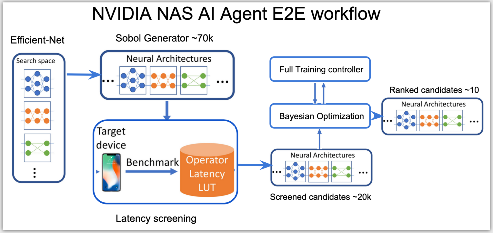
In the first stage, as the search space is high-dimensional, the agent uses Sobol sampling to distribute the candidates more evenly. Using the latency look-up table, these candidates are then categorized into a subsearch space, for example, a subset of networks with total latency under 0.5 msecs on NVIDIA V100 GPUs.
The inference latency used in this stage is an approximate cost, calculated by summing up the latency of each layer from the latency lookup table. The latency table uses input data shape and layer configurations as keys to look up the related latency on the queried layer.
In the second stage, the agent sets up Bayesian optimization loss function to find the best performing higher accuracy network within the latency range of the subspace:
Figure 2. NVIDIA NAS AI Agent End-to-End workflow
The AI agent uses a client-server distributed training controller to perform NAS simultaneously across multiple network architectures. The AI agent runs on one server node, proposing and training network candidates that run on several client nodes on the cluster.
Based on the results, only the promising network architecture candidates that meet both the accuracy and the latency targets of the target hardware get ranked, resulting in a handful of best-performing GPUNets that are ready to be deployed on NVIDIA GPUs using TensorRT.
GPUNet model architecture
The GPUNet model architecture is an eight-stage architecture using EfficientNet-V2 as the baseline architecture.
The search space definition includes searching on the following variables:
Type of operations
Number of strides
Kernel size
Number of layers
Activation function
IRB expansion ratio
Output channel filters
Squeeze excitation (SE)
Table 1 shows the range of values for each variable in the search space.
Table 1. Value ranges for search space variables
Stage
Type
Stride
Kernel
Layers
Activation
ER
Filters
SE
0
Conv
2
[3,5]
1
[R,S]
[24, 32, 8]
1
Conv
1
[3,5]
[1,4]
[R,S]
[24, 32, 8]
2
F-IRB
2
[3,5]
[1,8]
[R,S]
[2, 6]
[32, 80, 16]
[0, 1]
3
F-IRB
2
[3,5]
[1,8]
[R,S]
[2, 6]
[48, 112, 16]
[0, 1]
4
IRB
2
[3,5]
[1,10]
[R,S]
[2, 6]
[96, 192, 16]
[0, 1]
5
IRB
1
[3,5]
[0,15]
[R,S]
[2, 6]
[112, 224, 16]
[0, 1]
6
IRB
2
[3,5]
[1,15]
[R,S]
[2, 6]
[128, 416, 32]
[0, 1]
7
IRB
1
[3,5]
[0,15]
[R,S]
[2, 6]
[256, 832, 64]
[0, 1]
8
Conv1x1 & Pooling & FC
The first two stages search for the head configurations using convolutions. Inspired by EfficientNet-V2, the second and third stages use Fused-IRB. Fused-IRBs result in higher latency though, so in stages 4 to 7 these are replaced by IRBs.
The column Layers show the range of layers in the stage. For example, [1, 10] in stage 4 means that the stage can have 1 to 10 IRBs. The column Filters shows the range of output channel filters for the layers in the stage. This search space also tunes the expansion ratio (ER), activation types, kernel sizes, and the Squeeze Excitation (SE) layer inside the IRB/Fused-IRB.
Finally, the dimensions of the input image are searched from 224 to 512, at the step of 32.
Each GPUNet candidate build from the search space is encoded into a 41-wide integer vector (Table 2).
Table 2. The encoding scheme of networks in the search space
Stage
Type
Hyperparameters
Length
Resolution
[Resolution]
1
0
Conv
[#Filters]
1
1
Conv
[Kernel, Activation, #Layers]
3
2
Fused-IRB
[#Filters, Kernel, E, SE, Act, #Layers]
6
3
Fused-IRB
[#Filters, Kernel, E, SE, Act, #Layers]
6
4
IRB
[#Filters, Kernel, E, SE, Act, #Layers]
6
5
IRB
[#Filters, Kernel, E, SE, Act, #Layers]
6
6
IRB
[#Filters, Kernel, E, SE, Act, #Layers]
6
7
IRB
[#Filters, Kernel, E, SE, Act, #Layers]
6
At the end of the NAS search, the returned ranked candidates is a list of these best-performing encodings, which are in turn the best-performing GPUNets.
Summary
All ML practitioners are encouraged to read the CVPR 2022 GPUNet paper, with related GPUNet training code on the NVIDIA/DeepLearningExamples GitHub repo, and run inference on the colab instance on available cloud GPUs. GPUNet inference is also available on the PyTorch hub. The colab run instance uses the GPUNet checkpoints hosted on the NGC hub. These checkpoints have varying accuracy and latency tradeoffs, which can be applied based on the requirement of the target application.
Reinventing enterprise computing for the modern era, VMware CEO Raghu Raghuram Tuesday announced the availability of the VMware vSphere 8 enterprise workload platform running on NVIDIA DPUs, or data processing units, an initiative formerly known as Project Monterey. Placing the announcement in context, Raghuram and NVIDIA founder and CEO Jensen Huang discussed how running VMware Read article >
Multi-Instance GPU (MIG) is an important feature of NVIDIA H100, A100, and A30 Tensor Core GPUs, as it can partition a GPU into multiple instances. Each…
Multi-Instance GPU (MIG) is an important feature of NVIDIA H100, A100, and A30 Tensor Core GPUs, as it can partition a GPU into multiple instances. Each instance has its own compute cores, high-bandwidth memory, L2 cache, DRAM bandwidth, and media engines such as decoders.
This enables multiple workloads or multiple users to run workloads simultaneously on one GPU to maximize the GPU utilization, with guaranteed quality of service (QoS). A single A30 can be partitioned into up to four MIG instances to run four applications in parallel.
This post walks you through how to use MIG on A30 from partitioning MIG instances to running deep learning applications on MIG instances at the same time.
A30 MIG profiles
By default, MIG mode is disabled on the A30. You must enable MIG mode and then partition the A30 before any CUDA workloads can be run on the partitioned GPU. To partition the A30, create GPU instances and then create corresponding compute instances.
A GPU instance is a combination of GPU slices and GPU engines (DMAs, NVDECs, and so on). A GPU slice is the smallest fraction of the GPU that combines a single GPU memory slice and a single streaming multiprocessor (SM) slice.
Within a GPU instance, the GPU memory slices and other GPU engines are shared, but the SM slices could be further subdivided into compute instances. A GPU instance provides memory QoS.
You can configure an A30 with 24 GB of memory to have:
One GPU instance, with 24 GB of memory
Two GPU instances, each with 12 GB of memory
Three GPU instances, one with 12 GB of memory and two with 6 GB
Four GPU instances, each with 6 GB of memory
A GPU instance could be further divided into one or more compute instances depending on the size of the GPU instance. A compute instance contains a subset of the parent GPU instance’s SM slices. The compute instances within a GPU instance share memory and other media engines. However, each compute instance has dedicated SM slices.
For example, you could divide an A30 into four GPU instances, each having one compute instance, or divide an A30 into two GPU instances, each having two compute instances. Although both partitions result in four compute instances that can run four applications at the same time, the difference is that memory and other engines are isolated at the GPU instance level, not at the compute instance level. Therefore, if you have more than one user to share an A30, it is better to create different GPU instances for different users to guarantee QoS.
Table 1 provides an overview of the supported MIG profiles on A30, including the five possible MIG configurations that show the number of GPU instances and the number of GPU slices in each GPU instance. It also shows how hardware decoders are partitioned among the GPU instances.
Config
GPC Slice #0
GPC Slice #1
GPC Slice #2
GPC Slice #3
OFA
NVDEC
NVJPG
P2P
GPU Direct RDMA
1
4
1
4
1
No
Supported MemBW proportional to the size of the instance
2
2
2
0
2+2
0
No
3
2
1
1
0
2+1+1
0
No
4
1
1
2
0
1+1+2
0
No
5
1
1
1
1
0
1+1+1+1
0
No
Table 1. The MIG profiles supported on A30
GPC (graphics processing cluster) or slice represents a grouping of the SMs, caches, and memory. The GPC maps directly to the GPU instance. OFA (Optical Flow Accelerator) is an engine on the GA100 architecture on which A100 and A30 are based. Peer-to-peer (P2P) is disabled.
Table 2 provides profile names of the supported MIG instances on A30, and how the memory, SMs, and L2 cache are partitioned among the MIG profiles. The profile names for MIG can be interpreted as its GPU instance’s SM slice count and its total memory size in GB. For example:
MIG 2g.12gb means that this MIG instance has two SM slices and 12 GB of memory
MIG 4g.24gb means that this MIG instance has four SM slices and 24 GB of memory
By looking at the SM slice count of 2 or 4 in 2g.12gb or 4g.24gb, respectively, you know that you can divide that GPU instance into two or four compute instances. For more information, see Partitioning in the MIG User Guide.
Profile
Fraction of memory
Fraction of SMs
Hardware units
L2 cache size
Number of instances available
MIG 1g.6gb
1/4
1/4
0 NVDECs /0 JPEG /0 OFA
1/4
4
MIG 1g.6gb+me
1/4
1/4
1 NVDEC /1 JPEG /1 OFA
1/4
1 (A single 1g profile can include media extensions)
MIG 2g.12gb
2/4
2/4
2 NVDECs /0 JPEG /0 OFA
2/4
2
MIG 4g.24gb
Full
4/4
4 NVDECs /1 JPEG /1 OFA
Full
1
Table 2. Supported GPU instance profiles on A30 24GB
MIG 1g.6gb+me: me means media extensions to get access to the video and JPEG decoders when creating the 1g.6gb profile.
MIG instances can be created and destroyed dynamically. Creating and destroying does not impact other instances, so it gives you the flexibility to destroy an instance that is not being used and create a different configuration.
Manage MIG instances
Automate the creation of GPU instances and compute instances with the MIG Partition Editor (mig-parted) tool or by following the nvidia-smi mig commands in Getting Started with MIG.
The mig-parted tool is highly recommended, as it enables you to easily change and apply the configuration of the MIG partitions each time without issuing a sequence of nvidia-smi mig commands. Before using the tool, you must install the mig-parted tool following the instructions or grab the prebuilt binaries from the tagged releases.
Here’s how to use the tool to partition the A30 into four MIG instances of the 1g.6gb profile. First, create a sample configuration file that can then be used with the tool. This sample file includes not only the partitions discussed earlier but also a customized configuration, custom-config, that partitions GPU 0 to four 1g.6gb instances and GPU 1 to two 2g.12gb instances.
Next, apply the all-1g.6gb configuration to partition the A30 into four MIG instances. If MIG mode is not already enabled, then mig-parted enables MIG mode and then creates the partitions:
You can easily pick other configurations or create your own customized configurations by specifying the MIG geometry and then using mig-parted to configure the GPU appropriately.
After creating the MIG instances, now you are ready to run some workloads!
Deep learning use case
You can run multiple deep learning applications simultaneously on MIG instances. Figure 1 shows four MIG instances (four GPU instances, each with one compute instance), each running a model for deep learning inference, to get the most out of a single A30 for four different tasks at the same time.
For example, you could have ResNet50 (image classification) on instance one, EfficientDet (object detection) on instance two, BERT (language model) on instance three, and FastPitch (speech synthesis) on instance four. This example can also represent four different users sharing the A30 at the same time with ensured QoS.
Figure 1. A single A30 with four MIG instances running four models for inference simultaneously
Performance analysis
To analyze the performance improvement of A30 with and without MIG enabled, we benchmarked the fine-tuning time and throughput of the BERT PyTorch model for SQuAD (question answering) in three different scenarios on A30 (with and without MIG), also on T4.
A30 four MIG instances, each has a model, in total four models fine-tuning simultaneously
A30 MIG mode disabled, four models fine-tuning in four containers simultaneously
A30 MIG mode disabled, four models fine-tuning in serial
T4 has four models fine-tuning in serial
Fine-tune BERT base, PyTorch, SQuAD, BS=4
1
2
3
4
Result
A30 MIG: four models on four MIG devices simultaneously
Time (sec)
5231.96
5269.44
5261.70
5260.45
5255.89 (Avg)
Sequences/sec
33.88
33.64
33.69
33.70
134.91(Total)
A30 No MIG: four models in four containers simultaneously
Time (sec)
7305.49
7309.98
7310.11
7310.38
7308.99 (Avg)
Sequences/sec
24.26
24.25
24.25
24.25
97.01(Total)
A30 No MIG: four models in serial
Time (sec)
1689.23
1660.59
1691.32
1641.39
6682.53 (Total)
Sequences/sec
104.94
106.75
104.81
108.00
106.13(Avg)
T4: four models in serial
Time (sec)
4161.91
4175.64
4190.65
4182.57
16710.77(total)
Sequences/sec
42.59
42.45
42.30
42.38
42.43(Avg)
Table 3. Inference time (sec) and throughput (sequences/sec) for the four cases
To run this example, use the instructions in Quick Start Guide and Performance benchmark sections in the NVIDIA/DeepLearningExamples GitHub repo.
Based on the experimental results in Table 3, A30 with four MIG instances shows the highest throughput and shortest fine-tuning time for four models in total.
Speedup of total fine-tuning time for A30 with MIG:
1.39x compared to A30 No MIG on four models simultaneously
1.27x compared to A30 No MIG on four models in serial
3.18x compared to T4
Throughput of A30 MIG
1.39x compared to A30 No MIG on four models simultaneously
1.27x compared to A30 No MIG on four models in serial
3.18x compared to T4
Fine-tuning on A30 with four models simultaneously without MIG can also achieve high GPU utilization, but the difference is that there is no hardware isolation such as MIG provides. It incurs overhead from context switching and leads to lower performance compared to using MIG.
What’s next?
Built on the latest NVIDIA Ampere Architecture to accelerate diverse workloads such as AI inference at scale, A30 MIG mode enables you to get the most out of a single GPU and serve multiple users at the same time with quality of service.
No one likes standing around and waiting for the bus to arrive, especially when you need to be somewhere on time. Wouldn’t it be great if you could predict…
No one likes standing around and waiting for the bus to arrive, especially when you need to be somewhere on time. Wouldn’t it be great if you could predict when the next bus is due to arrive?
At the beginning of this year, Armenian developer Edgar Gomtsyan had some time to spare, and he puzzled over this very question. Rather than waiting for a government entity to implement a solution, or calling the bus dispatchers to try to confirm bus arrival times, he developed his own solution. Based on machine learning, it predicts bus arrival times with a high degree of accuracy.
As it happens, Gomtsyan’s apartment faces the street where a bus stop is located. To track the arrival and departure of buses, he mounted a small security camera on his balcony that uses image recognition software. “Like in any complex problem, to come to an effective solution, the problem was separated into smaller parts,” Gomtsyan said.
His solution uses a Dahua IP camera. For video processing, he initially used Vertex AI which can be used for image and object detection, classification, and other needs. Due to concerns about possible network and electricity issues, he eventually decided to process the video stream details locally using an NVIDIA Jetson Nano. You can access various libraries and trained models in the jetson-inference repo on GitHub.
The Real Time Streaming Protocol (RTSP) connected details from the camera’s video stream to the Jetson Nano. Then, using imagenet for classification and one of the pretrained models in the GitHub repo, Gomtsyan was able to get basic classifications for the stream right away.
Figure 1. The router with PoE adapter and Jetson Nano (left) and the mounted Dahua IP camera (right)
For the training geeks in the crowd, things start to get interesting at this point. Using the pretrained model, Gomtsyan used his setup to take a screenshot from the video stream every time it detected a bus. His first model was ready with around 100 pictures.
But, as Gomtsyan admits, “To say that things were perfect at first would be wrong.” It became obvious to him that he needed more pictures to increase the precision of the model output. Once he had 300 pictures, “the system got better and better,” he said.
When he first shared the results of this project, his model had been trained with more than 1,300 pictures, and it detects both arriving and departing buses—even in different weather conditions. He was also able to distinguish between scheduled buses from buses that happened to arrive randomly. His model now includes three classes of image detection: an arriving bus, background (everything that is not a scheduled bus), and a departing bus.
As an example, if an ‘arriving bus’ class prediction is greater than or equal to 92% for 15 frames, then it records the arrival time to a local CSV file.
To improve the data collected, his system takes a screenshot from the stream every time it detects a bus. This helps with both future model retraining and finding false-positive detections.
Further, to overcome the limitations of storing the CSV file data locally, Gomtsyan opted to store the data in BigQuery using the Google IoT service. As he notes, storing the data in the cloud “gives a more flexible and sustainable solution that will cater to future enhancements.”
He used the information collected to create a model that will predict when the next bus will arrive using the Vertex AI regression service. Gomtsyan recommends watching the video below to learn how to set up the model.
Video 1. Learn how to build and train ML models with Vertex AI
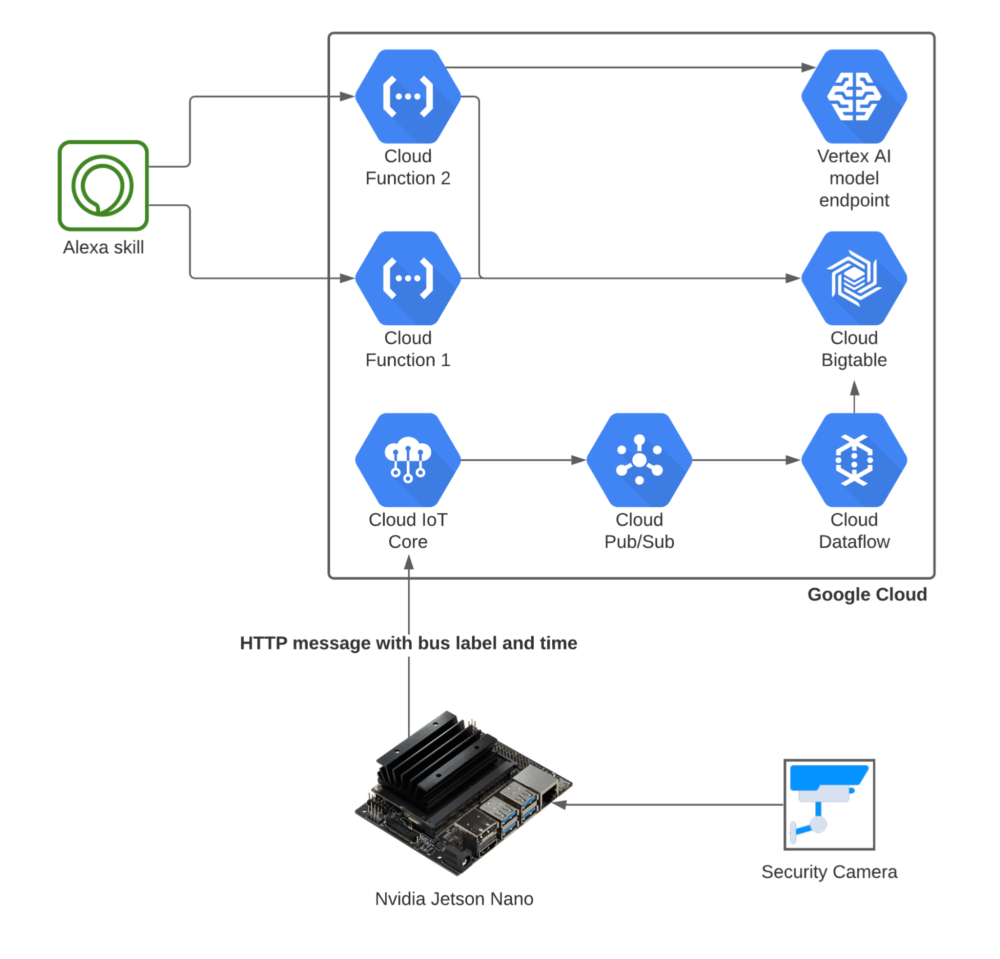
With a working model up and running, Gomtsyan needed an interface to let him know when the next bus should arrive. Rather than a website, he opted to use an IoT-based voice assistant. He originally planned to use Google Assistant for this purpose, but it was more challenging than expected. He instead used Alexa Skill, which is Amazon’s voice assistant tool. He created an Alexa Skill which queries respective cloud functions based on commands spoken to an Alexa speaker in his apartment.
Figure 2. The final architecture for Gomtsyan’s model
And while the predictions aren’t perfect, Gomtsyan has ideas for future enhancements that could help to improve the accuracy of the predicted bus arrival times, including traffic congestion data along the bus route. He is also considering using solar panels to power the system and make it autonomous, and introducing DevOps practices.
Gomtsyan developed this project to learn and challenge himself. Using his project documentation, other developers can replicate—and perhaps improve upon—his work. In the end, he hopes this bus prediction project will encourage others to pursue their ideas, “no matter how crazy, hard, or impossible they sound.”
Dell PowerEdge Servers Built With NVIDIA DPUs, NVIDIA GPUs and VMware vSphere 8 to Help Enterprises Boost AI Workload Performance and Build Foundation for Zero-Trust Security; Available to …
Doctors could soon evaluate Parkinson’s disease by having patients do one simple thing—sleep. A new study led by MIT researchers trains a neural network to…
Doctors could soon evaluate Parkinson’s disease by having patients do one simple thing—sleep. A new study led by MIT researchers trains a neural network to analyze a person’s breathing patterns while sleeping and determine whether the subject has Parkinson’s. Recently published in Nature Medicine, the work could lead to earlier detection and treatment.
“Our goal was to create a method for detecting and assessing Parkinson’s disease in a reliable and convenient way. Inspired by the connections between Parkinson’s and breathing signals, which are high-dimensional and complex, a natural choice was to use the power of machine learning to diagnose and track the progression,” said lead author Yuzhe Yang, a PhD student at MIT’s Computer Science & Artificial Intelligence Laboratory.
While notoriously difficult to pinpoint, Parkinson’s has become the fastest-growing neurological disease globally. About one million people in the US and 10 million worldwide are living with it. Despite these numbers, there isn’t one specific test for a speedy or definitive diagnosis.
As a progressive disorder, Parkinson’s often begins with subtle symptoms such as a slight hand tremor. It affects the nervous system and eventually leads to uncontrollable movements, shaking, stiffness while walking, and balance issues. Over time speech can become slurred and facial expressions fade away.
Neurologists often review a patient’s symptoms and medical history and rely on ruling out other illnesses based on imaging and lab work before diagnosing Parkinson’s. But symptoms vary and mimic several other disorders, which can lead to misdiagnosis and a delay in medical treatment. Early detection could help patients receive medications that are more effective when administered during the onset of Parkinson’s.
According to the authors, a correlation between nocturnal breathing and Parkinson’s was noted in 1817 by James Parkinson. A British medical doctor, he was the first to describe six individuals with symptoms of the disease he called paralysis agitans, which was later renamed.
Other research also found that brain stem degeneration in areas controlling patient breath occurs years earlier than motor skills symptoms and could be an early indicator of the disease.
The researchers saw an opportunity to employ AI, a powerful tool for detecting patterns and helping with disease diagnosis. They trained a neural network to analyze breathing patterns and learn those indicative of Parkinson’s.
The study dataset sampled 757 Parkinson’s patients and 6,914 control subjects, totaling 120,000 hours of sleep over 11,964 nights. The team trained the neural network model on several NVIDIA TITAN Xp GPUs using the cuDDN-accelerated PyTorch deep learning framework.
Figure 1. Overview of the AI model for Parkinson’s disease diagnosis and disease severity prediction from nocturnal breathing signals
A large amount of data came from a wireless radio transmitter the researchers developed. Similar in appearance to a Wi-Fi router the device emits radio waves and captures changes in the environment, which includes the rise and fall of a person’s chest. A neural network analyzes the patterns and determines whether Parkinson’s is present in the sample.
The AI model, deployed using NVIDIA TITAN Xp GPUs, is nearly 80% accurate in detecting Parkinson’s cases and 82% accurate in making a negative diagnosis. The algorithms can also determine the severity of Parkinson’s and track disease progression over time.
The work has the potential to speed up drug development with the newly found digital biomarkers for both diagnostics and tracking progression. Using AI models capable of detecting subtle patient changes and responses to new therapeutics could accelerate clinical trials, reduce costs, and inform more effective treatments.
It could also offer more accessible and equitable health care options to people beyond urban centers where specialists often practice medicine.
According to Yang, the team hopes to make the model more robust and accurate by collecting and testing data on more diverse populations and patients globally. They also envision use cases for the model to detect diseases beyond Parkinson’s.
“We believe there are chances to apply the method to detect other neurological diseases, for example, Alzheimer’s disease. The key problem is we need to collect a large and diverse dataset to carry out model training and evaluation for rigorous validation,” said Yang.
Contact pd-breathing@mit.edu for information about access to the code for noncommercial purposes.
Sign up for the latest Speech AI news from NVIDIA. Automatic speech recognition (ASR) is becoming part of everyday life, from interacting with digital…
Automatic speech recognition (ASR) is becoming part of everyday life, from interacting with digital assistants to dictating text messages. ASR research continues to progress, thanks to recent advances in:
ASR model multiple architectures to match needs
Customization flexibility in industry-specific jargon, languages, accents, and dialects
Cloud, on-prem, or hybrid deployment options
This post first introduces common ASR applications, and then features two startups exploring unique applications of ASR as a core product capability.
How speech recognition systems work
Automatic speech recognition, or speech recognition, is the capability of a computer system to decipher spoken words and phrases from audio and transcribe them into written text. Developers may also refer to ASR as speech-to-text, not to be confused with text-to-speech (TTS).
The text output of an ASR system may be the final product for a speech AI interface, or a conversational AI system may consume the text.
Common ASR applications
ASR has already become the gateway to novel interactive products and services. Even now you may be able to think of brand-name systems leveraging the use cases detailed below:
Live captioning and transcription
Live captioning and transcription are siblings. The main distinction between the two is that captioning produces subtitleslive, as needed, for video programs like streaming movies. By contrast, transcription may take place live or in batch mode, where recorded audio cuts are transcribed orders of magnitude faster than in real time.
Virtual assistants and chatbots
Virtual assistants and chatbots interact with people both to help and to entertain. They can receive text-based input from users typing or from an ASR system as it recognizes and outputs a user’s words.
Assistants and bots need to issue a response to the user quickly enough, so the processing delay is imperceptible. The response might be plain text, synthesized speech, or images.
Voice commands and dictation
Voice commands and dictation systems are common ASR applications used by social media platforms and in the healthcare industry.
To provide a social media example, before recording a video on a mobile device, a user might speak a voice command to activate beauty filters: “Give me purple hair.” This social networking application involves an ASR-enabled subsystem that receives a user’s words in the form of a command, while the application simultaneously processes camera input and applies filters for screen display.
Dictation systems store text from speech, expanding the vocabulary of the Speech AI system beyond commands. To provide an example from the healthcare industry, a doctor dictates voice notes packed with medical terminology and names. The accurate text output can be added to a visit summary in a patient’s electronic medical record.
Unique ASR applications
Beyond these common use cases, researchers and entrepreneurs are exploring a variety of unique ASR applications. The two startups featured below are developing products that use the technology in novel ways.
Interactive learning: Tarteel AI
Creative applications of ASR are beginning to appear in education materials, especially in the form of interactive learning, for both children and adults.
Tarteel.ai is a startup that has developed a mobile app using NVIDIA Riva to aid people in reciting and memorizing the Quran. (‘Tarteel’is the term used to define the recitation of the Quran in Arabic using melodic, beautiful tones.) The app applies an ASR model fine-tuned by Tarteel to Quranic Arabic. To learn more, watch the demo video in the social media post below.
As the screenshot of the app shows, a user sees the properly recited text, presented from right to left, top to bottom. The script in green is the word just spoken by the user (the leading edge). If a mistake happens in the recitation, the incorrect or missed words are marked in red and a counter keeps track of the inaccuracies for improvement.
The user’s progress is summarized with a list of recitation errors, including links to similar passages that may help the user remember the text. Challenge modes propel the user’s studies forward.
Challenges and solutions
While the app works smoothly now, Tarteel faced a tough set of initial challenges. To start, no suitable ASR model existed for Quranic Arabic, initially forcing Tarteel to try a general-purpose ASR model.
“We started with on-device speech AI frameworks, like for smartphones, but they were designed more for commands and short sentences than precise recitations,” co-founder and CEO of Tarteel Anas Abou Allaban said. “They also weren’t production-level tools—not even close.”
To overcome the challenge, Tarteel built a custom dataset to refine an existing ASR model to meet the app’s performance goals. Then, in their next prototype, the ASR model did perform with a lower word error rate (WER), but it still did not meet the app’s practical accuracy and latency requirements.
Allaban notes that he has seen 10-15% WER for some conference call transcripts, but it is another matter to see a high WER in Quranic studies. A processing latency longer than 300 milliseconds in the app “becomes very annoying,” he said.
Tarteel addressed these challenges by adjusting their ASR model in the NVIDIA NeMo framework and further optimizing its latency with TensorRT before deployment with Riva on Triton Inference Servers.
Digital human services: Ex-human
The startup Ex-human is creating hyper-realistic digital humansto interact with analog humans (you and me). Their current focus is developing a B2B digital human service for the entertainment niche, enabling the creation of chat bots or game characters with unique personalities, knowledge, and realistic speaking voices.
In the company’s Botify AI app, the AI entities include famous personalities to engage with users through verbal and graphical interactions, whether you’re typing in a smartphone chat window or using your voice. NVIDIA Riva Automatic Speech Recognition provides text input to the digital human’s natural language processing subsystems, comprised as part of a large language model (LLM).
Accurate and fast ASR is required to make virtual interactions believable. Because LLMs are compute-intensive and require ample processing resources, they could run too slowly for the interaction.
For example, Botify AI applies state-of-the-art TTS to produce a speech audio response which, in turn, drives facial animation using another AI model. The team has observed that a bot’s believable interactions with users are at their best when the turnaround time for a response is shorter than about a third of a second.
Challenges and solutions
While Botify AI is working to bridge the gap between realistic videos of AI-generated humans and real humans, the Ex-human team was surprised by an analysis of their customers’ behavioral data. “They’re building their own novel anime characters,” said Artem Rodichev, founder and CEO of Ex-human.
Employing ASR models fine-tuned for the Botify AI ecosystem, users may communicate with their favorite personalities or create their own. The surprising pattern of building novel anime characters emerged in the context of uploading custom faces to bring conversation to life with a custom persona. Rodichev explained that his team needed to quickly adapt their AI models to handle, for example, mouths that are stylistically just a dot or a line.
Rodichev and the team overcame many challenges in the architecture of Ex-human through the careful choice of tools and SDKs, as well as evaluating opportunities to parallelize processing. Rodichev cautions, “Because latency is so important, we optimized our ASR model and other models with NVIDIA TensorRT and rely on Triton Inference Server.”
Are Botify AI users ready to engage with digital humans more than with analog humans? Data reveals that users spend an average of 40 minutes a day with Botify AI digital humans, texting their favorites hundreds of messages during that time.
Get started with ASR
You can start including ASR capabilities in your own designs and projects, from hands-free voice commands to real-time transcription. Advanced SDKs such as Riva see high performance in world-class accuracy, speed, latency, and ease of integration—all aligned to enable your new idea.
Every AI application needs a strong inference engine. Whether you’re deploying an image recognition service, intelligent virtual assistant, or a fraud…
Every AI application needs a strong inference engine. Whether you’re deploying an image recognition service, intelligent virtual assistant, or a fraud detection application, a reliable inference server delivers fast, accurate, and scalable predictions with low latency (low response time to a single query) and strong throughput (large number of queries processed in a given time interval). Yet, checking all these boxes can be difficult and expensive to achieve.
Teams need to consider deploying applications that can leverage:
Diverse frameworks with independent execution backends (ONNX Runtime, TensorFlow, PyTorch)
Different inference types (real-time, batch, streaming)
Disparate inference serving solutions for mixed infrastructure (CPU, GPU)
Different model configuration settings (dynamic batching, model concurrency) that can significantly impact inference performance
These requirements can make AI inference an extremely challenging task, which can be simplified with NVIDIA Triton Inference Server.
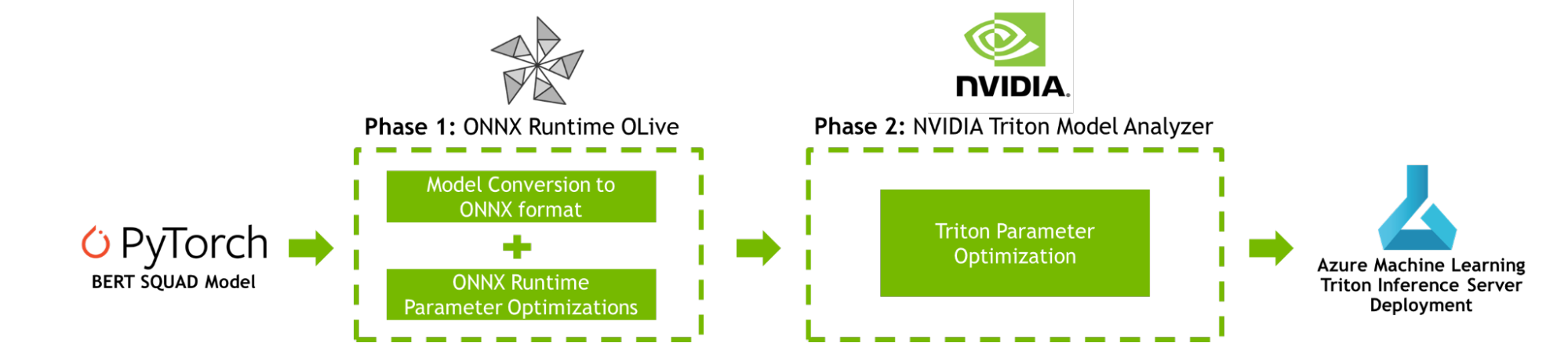
This post provides a step-by-step tutorial for boosting your AI inference performance on Azure Machine Learning using NVIDIA Triton Model Analyzer and ONNX Runtime OLive, as shown in Figure 1.
Figure 1. Workflow to optimize a PyTorch model using ONNX Runtime with OLive, Triton Model Analyzer, and Azure Machine Learning
Machine learning model optimization workflow
To improve AI inference performance, both ONNX Runtime OLive and Triton Model Analyzer automate the parameter optimization steps prior to model deployment. These parameters define how the underlying inference engine will perform. You can use these tools to optimize the ONNX Runtime parameters (execution provider, session options, and precision parameters), and the Triton parameters (dynamic batching and model concurrency parameters).
Phase 1: ONNX Runtime OLive optimizations
If Azure Machine Learning is where you deploy AI applications, you may be familiar with ONNX Runtime. ONNX Runtime is Microsoft’s high-performance inference engine to run AI models across platforms. It can deploy models across numerous configuration settings and is now supported in Triton. Fine-tuning these configuration settings requires dedicated time and domain expertise.
OLive (ONNX Runtime Go Live) is a Python package that speeds up this process by automating the work of accelerating models with ONNX Runtime. It offers two capabilities: converting models to ONNX format and auto-tuning ONNX Runtime parameters to maximize inference performance. Running OLive will isolate and recommend ONNX Runtime configuration settings for the optimal core AI inference results.
You can optimize an ONNX Runtime BERT SQuAD model with OLive using the following ONNX Runtime parameters:
Execution provider: ONNX Runtime works with different hardware acceleration libraries through its extensible Execution Providers (EP) framework to optimally run the ONNX models on the hardware platform, which can optimize the execution by taking advantage of the platform’s compute capabilities. OLive explores optimization on the following execution providers: MLAS (default CPU EP), Intel DNNL, and OpenVino for CPU, NVIDIA CUDA and TensorRT for GPU.
Session options: OLive sweeps through ONNX Runtime session options to find the optimal configuration for thread control, which includes inter_op_num_threads, intra_op_num_threads, execution_mode, and graph_optimization_level.
Precision: OLive evaluates performance with different levels of precision, including float32 and float16, and returns the optimal precision configuration.
After running through the optimizations, you still may be leaving some performance on the table at application level. The end-to-end throughput and latency can be further improved using the Triton Model Analyzer, which is capable of supporting optimized ONNX Runtime models.
Phase 2: Triton Model Analyzer optimizations
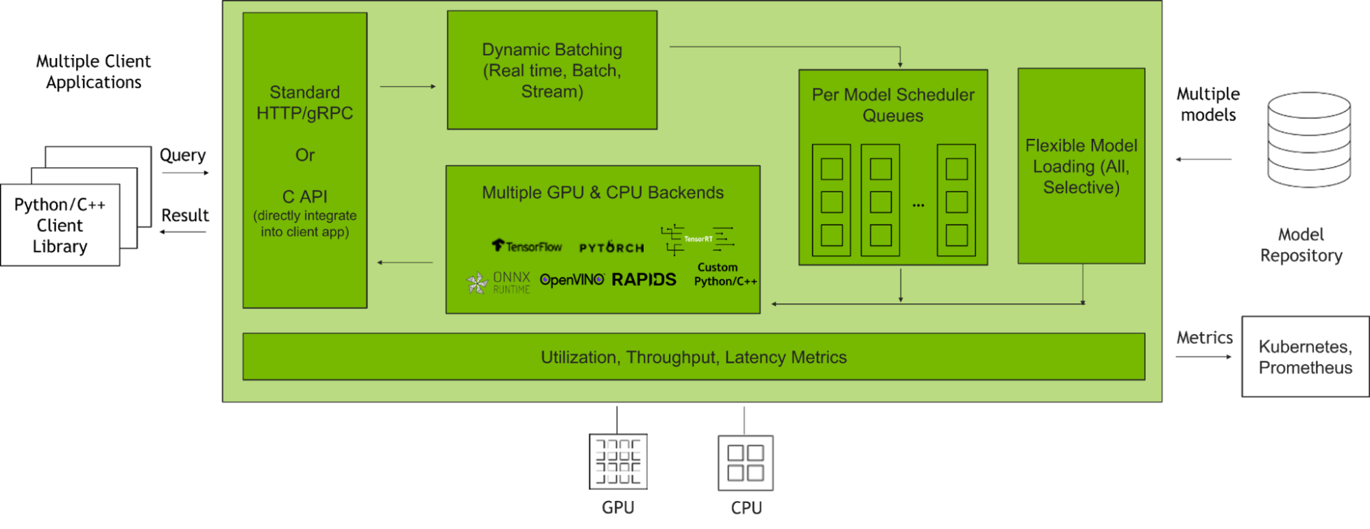
NVIDIA Triton Inference Server is an open-source inference serving software that helps standardize model deployment and execution and delivers fast and scalable AI inferencing in production. Figure 2 shows how the Triton Inference Server manages client requests when integrated with client applications and multiple AI models.
Figure 2. How the Triton Inference Server manages client requests
This post will focus on optimizing two major Triton features with Triton Model Analyzer:
Dynamic Batching: Triton enables inference requests to be combined by the server, so that a batch is created dynamically. This results in increased throughput within a fixed latency budget.
Model Concurrency: Triton allows multiple models or instances of the same model to execute in parallel on the same system. This results in increased throughput.
These features are extremely powerful when deployed at optimal levels. When deployed with suboptimal configurations, performance is compromised, leaving end applications vulnerable to current demanding quality-of-service standards (latency, throughput, and memory requirements).
As a result, optimizing batch size and model concurrency levels based on expected user traffic is critical to unlock the full potential of Triton. These optimized model configuration settings will generate improved throughput under strict latency constraints, boosting GPU utilization when the application is deployed. This process can be automated using the Triton Model Analyzer.
Given a set of constraints including latency, throughput targets, or memory footprints, Triton Model Analyzer searches for and selects the best model configuration that maximizes inference performance based on different levels for batch size, model concurrency, or other Triton model configuration settings. When these features are deployed and optimized, you can expect to see incredible results.
Tutorial: Begin optimizing inference performance
Four steps are required to deploy optimized machine learning models with ONNX Runtime OLive and Triton Model Analyzer on Azure Machine Learning:
Launch an Azure Virtual Machine with the NVIDIA GPU-optimized Virtual Machine Image (VMI)
Execute ONNX Runtime OLive and Triton Model Analyzer parameter optimizations on your model
Analyze and customize the results
Deploy the optimized Triton-ONNX Runtime model onto an Azure Machine Learning endpoint
To work through this tutorial, ensure you have an Azure account with access to NVIDIA GPU-powered virtual machines. For example, use Azure ND A100 v4-series VMs for NVIDIA A100 GPUs, NCasT4 v3-series for NVIDIA T4 GPUs, or NCv3-series for NVIDIA V100 GPUs. While the ND A100 v4-series is recommended for maximum performance at scale, this tutorial uses a standard NC6s_v3 virtual machine using a single NVIDIA V100 GPU.
Step 1: Launching an Azure virtual machine with NVIDIA’s GPU-optimized VMI
This tutorial uses the NVIDIA GPU-optimized VMI available on the Azure Marketplace. It is preconfigured with NVIDIA GPU drivers, CUDA, Docker toolkit, Runtime, and other dependencies. Additionally, it provides a standardized stack for developers to build their AI applications.
To maximize performance, this VMI is validated and updated quarterly by NVIDIA with the newest drivers, security patches, and support for the latest GPUs.
Step 2: Executing ONNX Runtime OLive and Triton Model Analyzer optimizations
Once you have connected to your Azure VM using SSH with the NVIDIA GPU-optimized VMI loaded, you are ready to begin executing ONNX Runtime OLive and Triton Model Analyzer optimizations.
First, clone the GitHub Repository and navigate to the content root directory by running the following commands:
git clone https://github.com/microsoft/OLive.git
cd OLive/olive-model_analyzer-azureML
Next, load the Triton Server container. Note that this tutorial uses the version number 22.06.
docker run --gpus=1 --rm -it -v “$(pwd)”:/models nvcr.io/nvidia/tritonserver:22.06-py3 /bin/bash
Once loaded, navigate to the /models folder where the GitHub material is mounted:
cd /models
Download the OLive and ONNX Runtime packages, along with the model you want to optimize. Then, specify the location of the model you want to optimize by setting up the following environmental variables:
You may adjust the location and file name provided above with a model of your choice. For optimal performance, download certified pretrained models directly from the NGC catalog. These models are trained to high accuracy and are available with high-level credentials and code samples.
The parameters in_names, in_shapes, and in_types refer to the names, shapes and types of the expected inputs for the model. In this case, inputs are sequences of length 256, however they are specified as [-1,256] to allow the batching of inputs. You can change the parameters values that correspond to your model and its expected inputs and outputs.
Now, you’re ready to run the pipeline by executing the following command:
This command first installs all necessary libraries and dependencies, and calls on OLive to convert the original model into an ONNX format.
Next, Triton Model Analyzer is called to automatically generate the model’s configuration file with the model’s metadata. The configuration file is then passed back into OLive to optimize via the ONNX Runtime parameters discussed earlier (execution provider, session options, and precision).
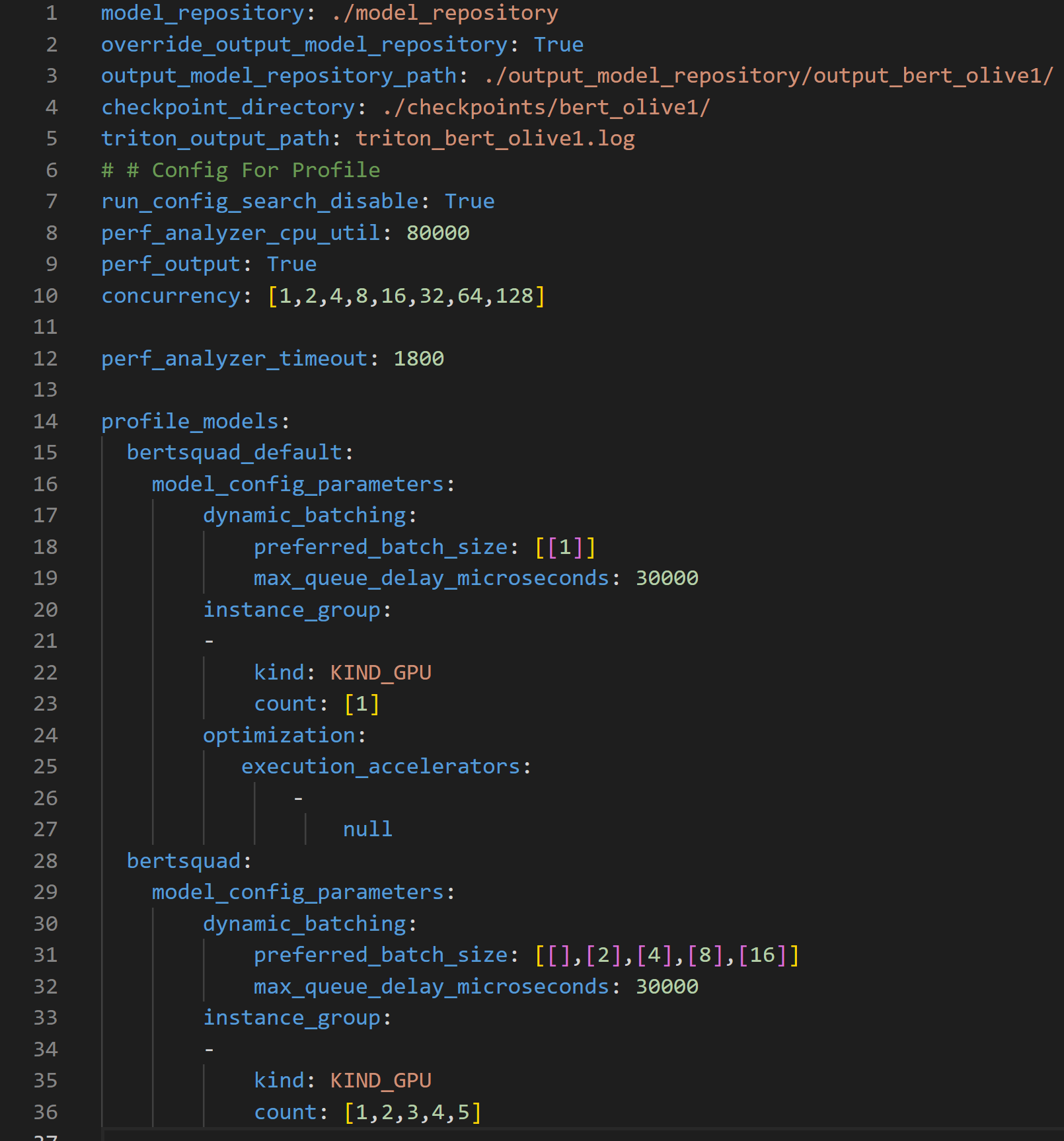
To further boost throughput and latency, the ONNX Runtime-optimized model configuration file is then passed into the Triton model repository for use by the Triton Model Analyzer tool. Triton Model Analyzer then runs the profile command, which sets up the optimization search space and specifies the location of the Triton Model repository using a .yaml configuration file (see Figure 3).
Figure 3. Profile configuration file outlining the Triton Model Analyzer search space to optimize inference performance
The configuration file above can be used to customize the search space for Triton Model Analyzer in a number of ways. The file requires the location of the Model Repository, parameters to optimize, and their ranges to create the search space used by Triton Model Analyzer to find the optimal configuration settings.
Lines 1-5 specify important paths, such as the location of the Output Model Repository where the optimized models are placed.
Line 10 specifies the parameter concurrency which dictates the concurrent inference request levels to be used by the Perf Analyzer, which emulates user traffic.
Line 15 specifies the bert_defaultmodel, which corresponds to the default model obtained from the PyTorch to ONNX conversion. This model is the baseline model and therefore uses non-optimized values for dynamic batching (line 17) and model concurrency (line 20)
Lines 19 and 32 shows a latency constraint of 30ms that must be satisfied during the optimization process.
Line 28 specifies the bertsquadmodel, which corresponds to the OLive optimized model. This one differs from the bert_default model because the dynamic batching parameter search space here is set to 1, 2, 4, 8 and 16, and the model concurrency parameter search space is set to 1, 2, 3, 4 and 5.
The profile command records results across each concurrent inference request level, and for each concurrent inference request level, the results are recorded for 25 different parameters since the search space for both the dynamic batching and model concurrency parameters have five unique values each, equating to a total of 25 different parameters. Note that the time needed to run this will scale with the number of configurations provided in the search space within the profile configuration file in Figure 3.
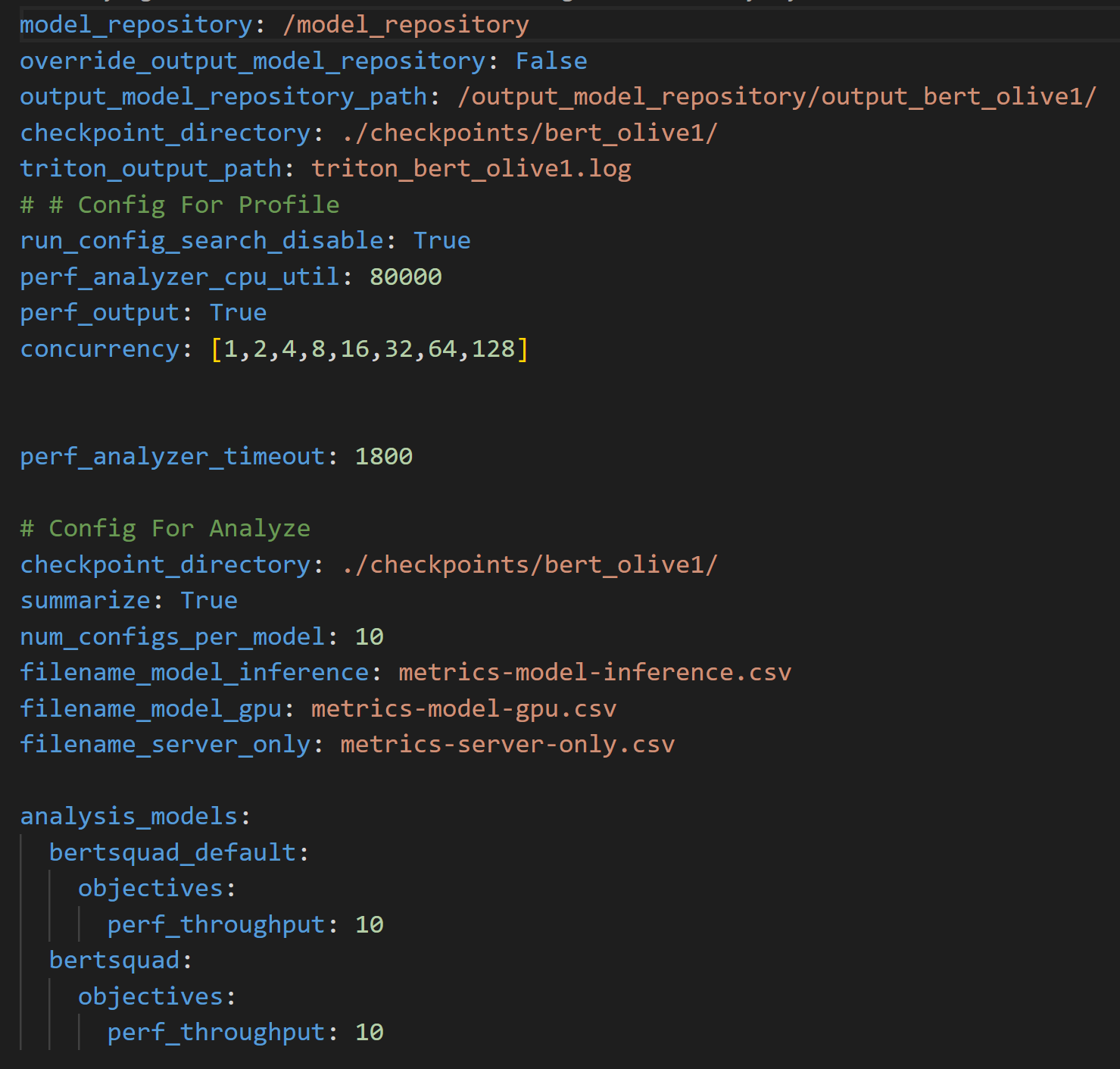
The script then runs the Triton Model Analyzer analyzecommand to process the results using an additional configuration file shown in Figure 4. The file specifies the location of the output model repository where the results were generated from the profile command, along with the name of the CSV files where the performance results will be recorded.
Figure 4. Analyze configuration file used to run the analyze command and process the results from the profile command
While the profile and analyze commands may take a couple of hours to run, the optimized model configuration settings will ensure strong long-term inference performance for your deployed model. For shorter run times, adjust the model profile configuration file (Figure 3) with a smaller search space across the parameters you wish to optimize.
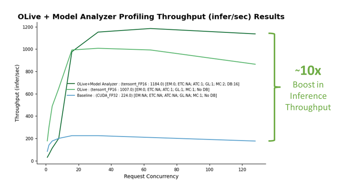
Once the demo completes running, there should be two files produced: Optimal_Results.png as shown in Figure 5, and Optimal_ConfigFile_Location.txt, which represents the location of the optimal config file to be deployed on Azure Machine Learning. A non-optimized baseline is established (blue line). The performance boost achieved through OLive optimizations is shown (light green line), along with OLive + Triton Model Analyzer optimizations (dark green line).
Step 3: Analyzing performance results
Figure 5. 10x boost in inference throughput when applying OLive plus Triton Model Analyzer optimized configuration settings on an Azure virtual machine (Standard_NC6s_v3) using a single V100 NVIDIA GPU. (Note: This is not an official benchmark.)
The baseline corresponds to a model with non-optimized ONNX Runtime parameters (CUDA backend with full precision) and non-optimized Triton parameters (no dynamic batching nor model concurrency). With the baseline established, it is clear there is a big boost in inference throughput performance (y-axis) obtained from both OLive and Triton Model Analyzer optimizations at various inference request concurrency levels (x-axis) emulated by Triton Perf Analyzer, a tool that mimics user traffic by generating inference requests.
OLive optimizations improved model performance (light green line) by tuning the execution provider to TensorRT with mixed precision, along with other ONNX Runtime parameters. However, this shows performance without Triton dynamic batching or model concurrency. Therefore, this model can be further optimized with Triton Model Analyzer.
Triton Model Analyzer further boosts inference performance by 20% (dark green line) after optimizing model concurrency and dynamic batching. The final optimal values selected by Triton Model Analyzer are a model concurrency of two (two copies of the BERT model will be saved on the GPU) and a maximum dynamic batching level of 16 (up to 16 inference requests will be batched together at one time).
Overall, the gain on inference performance using optimized parameters is more than 10x.
Additionally, if you are expecting certain levels of inference requests for your application, you may adjust the emulated user traffic by configuring the Triton perf_analyzer. You may also adjust the model configuration file to include additional parameters to optimize such as Delayed Batching.
You’re now ready to deploy your optimized model with Azure Machine Learning.
Step 4: Deploying the optimized model onto an Azure Machine Learning endpoint
Managed online endpoints help you deploy ML models in a turnkey manner. It takes care of serving, scaling, securing, and monitoring your models, freeing you from the overhead of setting up and managing the underlying infrastructure.
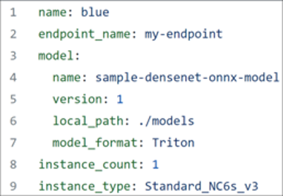
To continue, ensure you have downloaded the Azure CLI, and have at hand the YAML file shown in Figure 6.
Figure 6. YAML file for the optimized BERT model
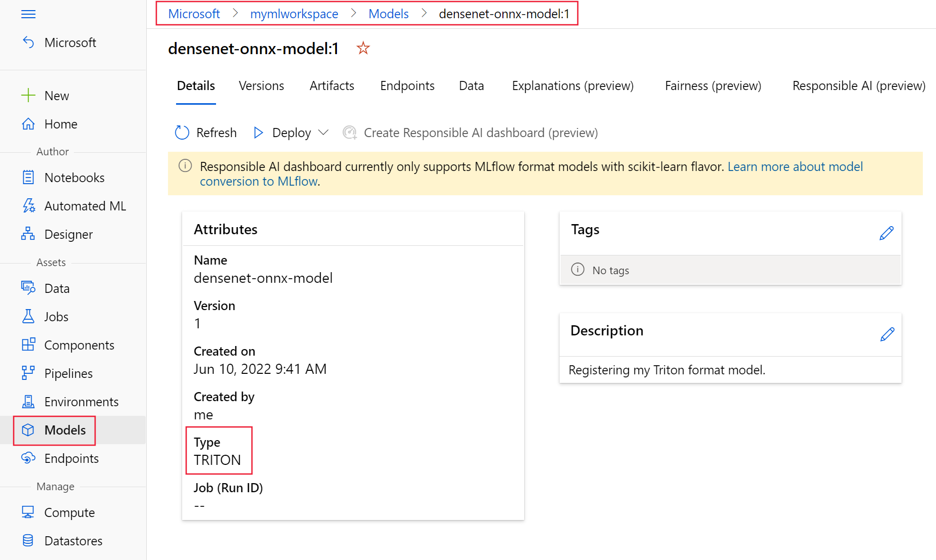
First, register your model in Triton format using the above YAML file. Your registered model should look similar to Figure 7 as shown on the Modelspage of Azure Machine Learning Studio.
Figure 7. Azure Machine Learning Studio registered optimized model
Next, select the Triton model, select ‘Deploy,’ and then ‘Deploy to real-time endpoint.’ Continue through the wizard to deploy the ONNX Runtime and Triton optimized model to the endpoint. Note that no scoring script is required when you deploy a Triton model to an Azure Machine Learning managed endpoint.
Congratulations! You have now deployed a BERT SQuAD model optimized for inference performance using ONNX Runtime and Triton parameters on Azure Machine Learning. By optimizing these parameters, you have unlocked a 10x increase in performance relative to the non-optimized baseline BERT SQuAD model.
Resources for exploring machine learning model inference tools
Explore more resources about deploying AI applications with NVIDIA Triton, ONNX Runtime, and Azure Machine Learning below:

 Crafted by AI for AI, GPUNet is a class of convolutional neural networks designed to maximize the performance of NVIDIA GPUs using NVIDIA TensorRT. Built using…
 Multi-Instance GPU (MIG) is an important feature of NVIDIA H100, A100, and A30 Tensor Core GPUs, as it can partition a GPU into multiple instances. Each…
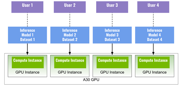
") No one likes standing around and waiting for the bus to arrive, especially when you need to be somewhere on time. Wouldn’t it be great if you could predict…
No one likes standing around and waiting for the bus to arrive, especially when you need to be somewhere on time. Wouldn’t it be great if you could predict…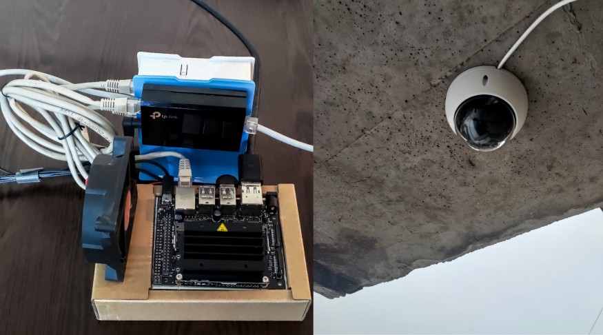
 Learn about the latest AI and data science breakthroughs from the world’s leading data science teams at GTC 2022.
 Doctors could soon evaluate Parkinson’s disease by having patients do one simple thing—sleep. A new study led by MIT researchers trains a neural network to…
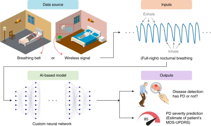
 Sign up for the latest Speech AI news from NVIDIA. Automatic speech recognition (ASR) is becoming part of everyday life, from interacting with digital…
 Every AI application needs a strong inference engine. Whether you’re deploying an image recognition service, intelligent virtual assistant, or a fraud…