
 NVIDIA Clara medical AI models can now run natively on MD.ai in the cloud, enabling collaborative model validation and rapid annotation projects using modern web browsers.
Medical imaging AI models built with NVIDIA Clara can now run natively on MD.ai in the cloud, which enables collaborative model validation and rapid annotation projects using modern web browsers. These NVIDIA Clara models are free to use in any MD.ai project for collaborative research, such as for organ or tumor segmentation.
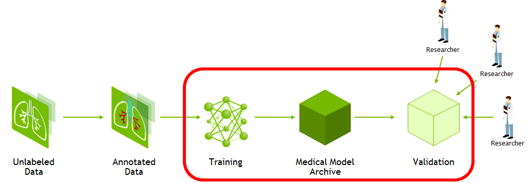
AI solutions have been shown to help streamline radiology and enterprise imaging workflows. However, the process to create, share, test, and scale computer vision models is not as streamlined for all modalities, conditions, and findings. Several critical components are needed to create robust models and support the most diverse acquisition devices and patient populations. These critical components can include the ability to create ground truth for unannotated imaging studies and the ability to collaborate worldwide to assess the use of models with validation data.
MD.ai’s real-time collaborative annotation platform and the NVIDIA Clara deep learning training framework are helping to create more robust model building and collaboration.
In this post, we walk through the basics of the Clara Train MMAR and the steps necessary to prepare it for use with MD.ai. In just a few steps, you can deploy any of these pretrained models on MD.ai for seamless web-based evaluation and collaboration. After they’re deployed on MD.ai, these models can be used in any existing or new MD.ai projects.
NVIDIA Clara Train
The Clara Train training framework is an application package built on the Python-based NVIDIA Clara Train SDK. This framework is designed to enable rapid implementation of deep learning solutions in medical imaging based on optimized, ready-to-use, pretrained medical imaging models built in-house by NVIDIA researchers.
The Clara Training framework uses a standard structure for models, the Medical Model Archive (MMAR), which contains the pretrained model as well as scripts that define end-to-end development workflows for training, fine-tuning, validation, and inference.
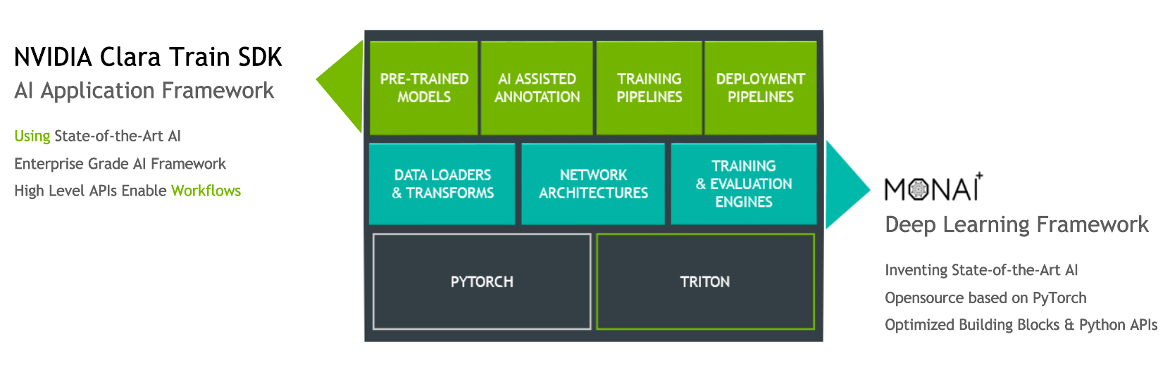
The Clara Train v4.0+ SDK uses a component-based architecture built on the open source, PyTorch-based framework MONAI (Medical Open Network for AI). MONAI provides domain-optimized foundational capabilities in healthcare imaging that can be used to build training workflows in a native PyTorch paradigm. The Clara Train SDK uses these foundational components such as optimized data loaders, transforms, loss functions, optimizers, and metrics to implement end-to-end training workflows packaged as MMARs.
MD.ai
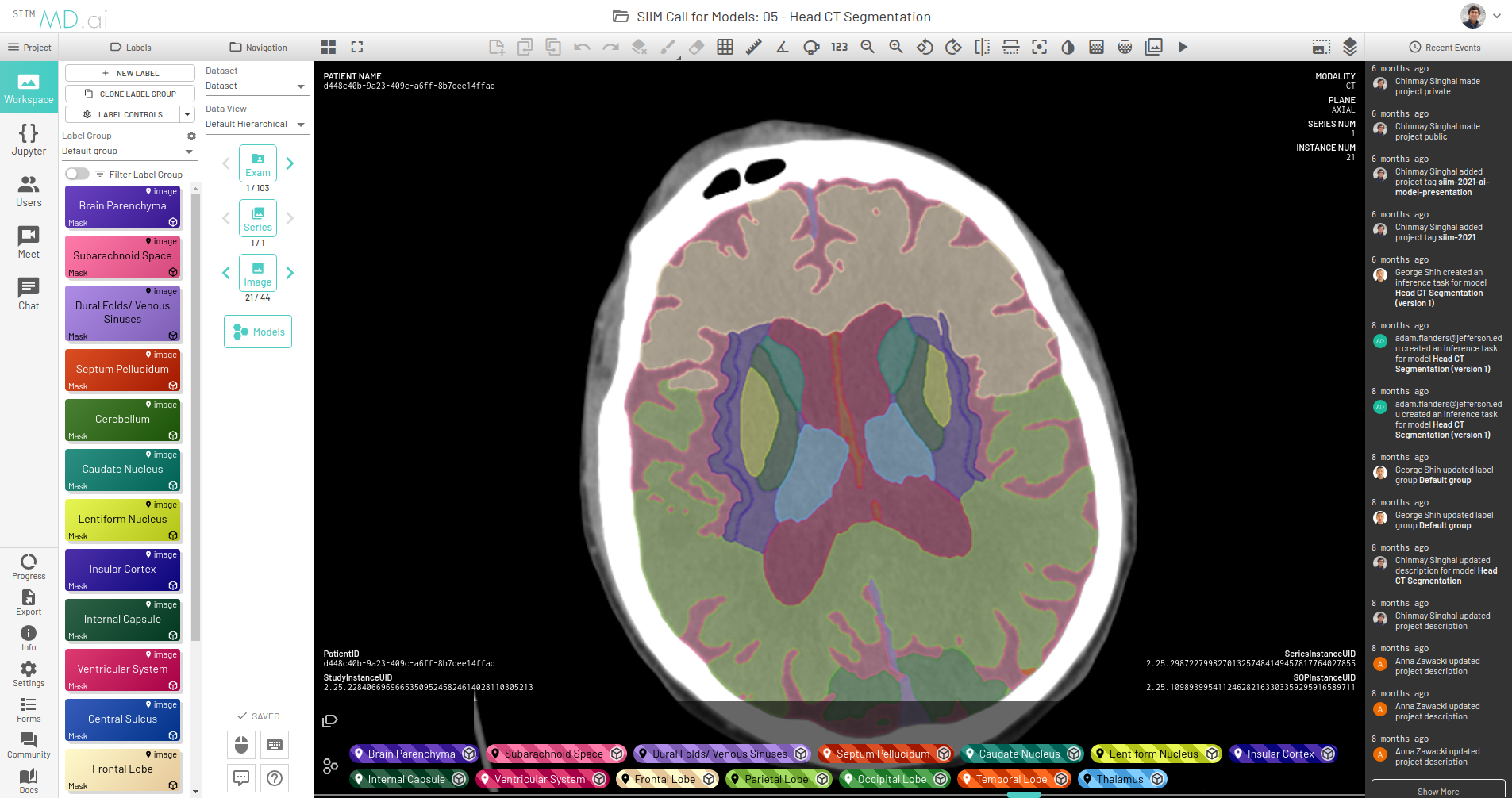
MD.ai provides a web-based and cloud native annotation platform that enables real-time collaboration among teams of clinicians and researchers, with shared workspaces. You can also load multiple deep learning models for real-time evaluation.
The platform provides an easy and seamless interface for dataset construction and AI project creation. It gives users a wide suite of tools for annotating data and building machine-learning algorithms to accelerate the application of AI in medicine, with a particular focus on medical imaging.
Coupling this capability with the ability to quickly deploy Clara Train model MMARs on the MD.ai platform gives you an end-to-end workflow that spans rapid model development, model training, fine-tuning, inference, and rapid evaluation and visualization. This end-to-end capability streamlines the process of taking a model from research and development to production.
Solution overview
The starting point for Clara Train is the NGC Clara Train Collection. Here, you find the Clara Train SDK container, a collection of freely available, pretrained models, and a collection of Jupyter notebooks that walk through the main concepts of the SDK. All the Clara Train models share the MMAR format mentioned earlier.
The Clara Train MMAR defines a standard structure for storing the files required for defining the model development workflow, as well the files produced when executing the model for validation and inference. This structure is defined as follows:
ROOT
    config
        config_train.json
        config_finetune.json
        config_inference.json
        config_validation.json
        config_validation_ckpt.json
        environment.json
    commands
        set_env.sh
        train.sh                        train with single GPU
        train_multi_gpu.sh              train with 2 GPUs
        finetune.sh                     transfer learning with CKPT
        infer.sh                        inference with TS model
        validate.sh                     validate with TS model
        validate_ckpt.sh                validate with CKPT
        validate_multi_gpu.sh           validate with TS model on 2 GPUs
        validate_multi_gpu_ckpt.sh      validate with CKPT on 2 GPUs
        export.sh                       export CKPT to TS model
    resources
        log.config
        ...
    docs
        license.txt
        Readme.md
        ...
    models
        model.pt
        model.ts
        final_model.pt
    eval
        all evaluation outputs: segmentation / classification results
        metrics reports, etc.
All pretrained models provided for use with Clara Train, as well as custom models developed with the Clara Train framework, use this structure. To prepare an MMAR for use with MD.ai, we assume a pretrained model and focus on a couple key components for deployment.
The first component is the environment.json file that defines the common parameters for the model, including dataset paths and model checkpoints. For example, the environment.json file from the Clara Train spleen segmentation task defines the following parameters:
{
   "DATA_ROOT": "/workspace/data/Task09_Spleen_nii",
   "DATASET_JSON": "/workspace/data/Task09_Spleen_nii/dataset_0.json",
   "PROCESSING_TASK": "segmentation",
   "MMAR_EVAL_OUTPUT_PATH": "eval",
   "MMAR_CKPT_DIR": "models",
   "MMAR_CKPT": "models/model.pt"
   "MMAR_TORCHSCRIPT": "models/model.ts"
}
When preparing the model for integration with MD.ai, make sure that the MMAR contains the trained MMAR_CKPT and MMAR_TORCHSCRIPT in the MMAR’s models/ directory. These are generated by executing the bundled train.sh and export.sh, respectively.
- The
train.shscript executes model training, which requiresDATA_ROOTandDATASET_JSONfor the input dataset and generates the MMAR_CKPT. - The
infer.shscript serializes this checkpoint into theMMAR_TORCHSCRIPTused for inference.
With a pretrained model, both the checkpoint and TorchScript are provided, and you can focus on the inference pipeline. Inference is executed using the MMAR’s infer.sh script:
1    #!/usr/bin/env bash
2    my_dir="$(dirname "$0")"
3    . $my_dir/set_env.sh
4    echo "MMAR_ROOT set to $MMAR_ROOT"
5
6    CONFIG_FILE=config/config_validation.json
7    ENVIRONMENT_FILE=config/environment.json
8    python3 -u  -m medl.apps.evaluate
9       -m $MMAR_ROOT
10       -c $CONFIG_FILE
11       -e $ENVIRONMENT_FILE
12       --set
13       DATASET_JSON=$MMAR_ROOT/config/dataset_0.json
14       output_infer_result=true
15       do_validation=false
This script runs inference on the validation subset, defined in config_validation.json, of the full dataset defined in environment.json. If reference test data is provided along with the MMAR, the paths to this data must be defined. When you integrate the MMAR, MD.ai handles the dataset directly, and these values are overridden as part of the integration.
To deploy your own pretrained AI models on MD.ai for inference, you must already have an existing project or create a new project on the platform. The project also must contain the dataset on which to test your model. For more information, see Set Up Project.
Next, to deploy your AI model, the inference code must be transformed into a specific format that is compatible with the platform. The following files are the bare minimum for a successful deployment:
config.yamlmdai_deploy.pyrequirements.txtmodel-weights
For more information about these files, see MD.ai Interface Code.
For NVIDIA Clara models, we have further streamlined this for you and there is no need to write these files from scratch. We provide skeleton codes for each different category of deep learning models supported by the NGC catalog: classification, segmentation, and so on. You can download the model-specific skeleton code, make a few adjustments that are outlined later in this post, and then upload the models on MD.ai for inference.
Inference steps
After you have an MMAR prepared, here’s how to use it directly for running the model on MD.ai. This post walks you through an example segmentation model that’s already deployed on the platform: the skeleton code for running segmentation models on MD.ai, which is actually the code for a CT spleen segmentation model from NVIDIA.
Now, to deploy the liver and tumor segmentation model using the same MMAR format, follow these steps:
- Download the skeleton code for segmentation models.
- Download the MMAR for the liver and tumor segmentation model from the NGC catalog.
- In the downloaded skeleton code, replace the
/workspace/clara_pt_spleen_ct_segmentation_1folder with your downloaded MMAR folder. - In the
/workspace/config_mdai.jsonfile, make the following changes:
1    {
2        “type” : “segmentation”,
3        “root_folder”: “clara_pt_spleen_ct_segmentation_1”,
4        “out_classes” : 2,
5        “data_list_key”: “test”
6    }
- root_folder—Replace this key value with the name of your downloaded MMAR folder, such as clara_pt_liver_and_tumor_ct_segmentation_1 for the liver and tumor example.
- out_classes—Replace this value with the number of output classes for your model, such as 3 in this case (background: 0, liver: 1, and tumor: 2).
- data_list_key—Replace with the key name mentioned in the data_list_key attribute of your MMAR’s config/config_inference.json file, such as testing.
- In the
/mdaifolder, make the following changes:
- In the
config.yamlfile, change theclara_versionkey to the appropriate version used by your model (for example, 3.1.01 or 4.0).
1    base_image: nvidia
2    clara_version: 4.0
3    device_type: gpu
- In
requirements.txt, add any additional dependencies required, more than those provided by the NVIDIA Clara base image and those already present in the file.
This prepares your model for deployment on MD.ai. Both the spleen and liver tumor segmentation models have been deployed on the MD.ai platform and are available for evaluation.
Similar steps can be done for classification models, though we are working towards further streamlining this integration. For the skeleton code for an example NVIDIA model that classifies chest X-rays into 15 abnormalities, see Example: NVIDIA MMAR for disease classification in chest x-rays on GitHub. This model is also deployed on the public site.
When the code is ready, it must be wrapped in a zip file so that it can be uploaded on MD.ai for inference. For more information, see Deploying models.
Your model is now ready to be tried within MD.ai on any dataset of your choice!
The best part is that all models need only be deployed one time on the MD.ai platform. As soon as an NVIDIA Clara model is deployed on MD.ai, it can be used in any MD.ai project by using the model cloning feature. Here’s an example of cloning the NVIDIA Liver Segmentation model into a new MD.ai project by just copying the value:
Future features
We are working towards streamlining the integration to minimize the steps required to deploy the MMAR, with plans to eliminate all code modification, so that deployment is as easy as just clicking a button.
MD.ai plans to predeploy all the models available on NGC so that you can use them directly by cloning from our public projects, saving you from the process of deploying MMARs on your own. We are also going to create NVIDIA Clara Starter Packs so that you can easily get started with selected models preattached to your project.
Another important plan is to add support for training AI models on MD.ai. When we have that, you can effectively use the NVIDIA AI-assisted annotation product on the platform to help users annotate much faster and much easier, rather than starting from scratch.
Summary
In this post, we highlighted key components of each platform and the steps necessary to quickly deploy a medical imaging model built with NVIDIA Clara on MD.ai.
Try out a live demo of the NVIDIA Clara Liver and Spleen Segmentation models in MD.ai. If you have any questions, contact hello@md.ai or claraimaging@nvidia.com.
 The new Amazon EC2 G5g instances feature the AWS Graviton2 processors and NVIDIA T4G Tensor Core GPUs, to power rich android game streaming for mobile devices.
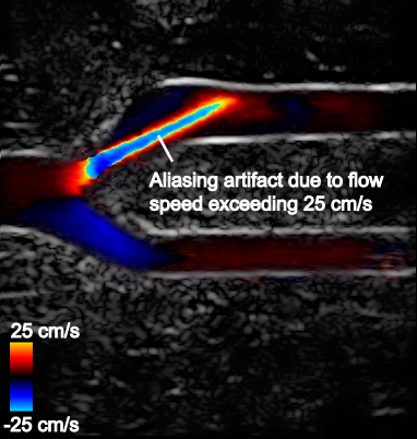
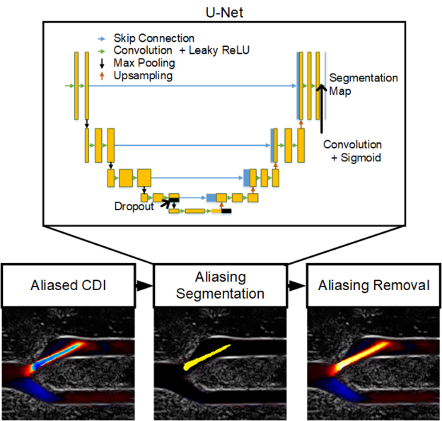
 The NVIDIA Clara developer kit, NVIDIA Clara Holoscan, and us4us front end help build AI models on streaming data for ultrasounds, to remove artifacts like aliasing.
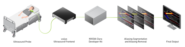
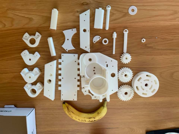
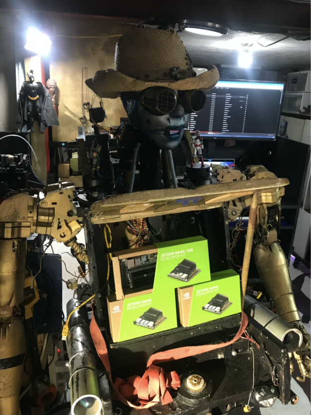
 This post features winners from the NVIDIA sponsored contest with Make: where makers submit their best robotics projects with a galactic theme.


 NVIDIA cuTENSOR, version 1.4, library supports 64-dimensional tensors, distributed multi-GPU tensor operations, and improves tensor contraction performance models.
 Project MONAI continues to expand its end-to-end workflow with new releases and a new component called MONAI Deploy Inference Service.