The first post in this series covered how to train a 2D pose estimation model using an open-source COCO dataset with the BodyPoseNet app in the NVIDIA Transfer Learning Toolkit. In this post, you learn how to optimize the pose estimation model in the NVIDIA Transfer Learning Toolkit. It walks you through the steps of … Continued
The first post in this series covered how to train a 2D pose estimation model using an open-source COCO dataset with the BodyPoseNet app in the NVIDIA Transfer Learning Toolkit.
In this post, you learn how to optimize the pose estimation model in the NVIDIA Transfer Learning Toolkit. It walks you through the steps of model pruning and INT8 quantization to optimize the model for inference.
Model optimizations and export
This section covers few topics of model optimization and export:
- Pruning
- INT8 quantization
- Best practices for improving speed and accuracy
Pruning
BodyPoseNet supports model pruning to remove unnecessary connections, reducing the number of parameters by an order of magnitude. This results in an optimized model architecture.
Prune the model
To prune the model, use the following command:
tlt bpnet prune -m $USER_EXPERIMENT_DIR/models/exp_m1_unpruned/bpnet_model.tlt
                 -o $USER_EXPERIMENT_DIR/models/exp_m1_pruned/bpnet_model.pruned-0.05.tlt
                 -eq union
                 -pth 0.05
                 -k $KEY
Usually, you just have to adjust -pth (threshold) for accuracy and model size trade off. For some internal studies, we’ve noticed that a pth value between the range [0.05, 3.0] is a good starting point for BodyPoseNet models.
Retrain the pruned model
After the model has been pruned, there might be a slight decrease in accuracy because some previously useful weights may have been removed. To regain the accuracy, we recommend retraining this pruned model over the same dataset. You can follow the same instructions as in the Train experiment configuration file section. The main change is now to specify pretrained_weights as the path to pruned model and enable load_graph. Because the model is being initialized with pruned model weights, the model converges faster.
# Retraining using the pruned model as model graph
 tlt bpnet train -e $SPECS_DIR/bpnet_retrain_m1_coco.yaml
                 -r $USER_EXPERIMENT_DIR/models/exp_m1_retrain
                 -k $KEY
                 --gpus $NUM_GPUS
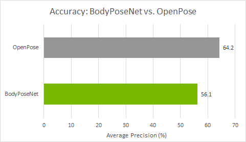
You can follow similar instructions as in the Evaluation and Model verification sections to evaluate and verify the pruned model. After retraining the pruned model with pth 0.05, you can observe an accuracy of 56.1% AP with multiscale inference. Here are the metrics on COCO validation set:
Average Precision  (AP) @[ IoU=0.50:0.95 | area=   all | maxDets= 20 ] = 0.561
Average Precision  (AP) @[ IoU=0.50      | area=   all | maxDets= 20 ] = 0.776
Average Precision  (AP) @[ IoU=0.75      | area=   all | maxDets= 20 ] = 0.609
Average Precision  (AP) @[ IoU=0.50:0.95 | area=medium | maxDets= 20 ] = 0.567
Average Precision  (AP) @[ IoU=0.50:0.95 | area= large | maxDets= 20 ] = 0.556
...
Export the .etlt model
Inference throughput and how quickly you can create an efficient model are two key metrics for deploying deep learning applications because they directly affect the time to market and the cost of deployment. TLT includes an export command to export and prepare TLT models for deployment.
The model is exported as a .etlt (encrypted TLT) file. The file is consumable by the TLT CV Inference, which decrypts the model and converts it to a TensorRT engine. Exporting the model decouples the training process from inference and allows conversion to TensorRT engines outside the TLT environment. TensorRT engines are specific to each hardware configuration and should be generated for each unique inference environment. The following code example shows the export of the pruned, retrained model.
tlt bpnet export -m $USER_EXPERIMENT_DIR/models/exp_m1_retrain/bpnet_model.tlt
                  -e $SPECS_DIR/bpnet_retrain_m1_coco.yaml
                  -o $USER_EXPERIMENT_DIR/models/exp_m1_final/bpnet_model.etlt
                  -k $KEY
                  -t tfonnx
The export command can optionally generate the calibration cache for running inference at INT8 precision. This is described more in detail in later sections.
INT8 quantization
The BodyPoseNet model supports int8 inference mode in TensorRT. To do this, the model is first calibrated to run 8-bit inferences. To calibrate the model, you need a directory with a sampled set of images to be used for calibration.
We’ve provided a helper script that parses the annotations and samples the required number of images at random based on specified criteria like number of people in the image, number of keypoints per person, and so on.
# Number of calibration samples to use
 export NUM_CALIB_SAMPLES=2000

 python3 sample_calibration_images.py
     -a $LOCAL_EXPERIMENT_DIR/data/annotations/person_keypoints_train2017.json
     -i $LOCAL_EXPERIMENT_DIR/data/train2017/
     -o $LOCAL_EXPERIMENT_DIR/data/calibration_samples/
     -n $NUM_CALIB_SAMPLES
     -pth 1
     --randomize
Generate INT8 calibration cache and engine
The following command exports the pruned, retrained model to the .etlt format, performs INT8 calibration, and generates the INT8 calibration cache and TensorRT engine for the current hardware.
# Set dimensions of desired output model for inference/deployment
 export IN_HEIGHT=288
 export IN_WIDTH=384
 export IN_CHANNELS=3
 export INPUT_SHAPE=288x384x3
 # Set input name
 export INPUT_NAME=input_1:0

 tlt bpnet export
     -m $USER_EXPERIMENT_DIR/models/exp_m1_retrain/bpnet_model.tlt
     -o $USER_EXPERIMENT_DIR/models/exp_m1_final/bpnet_model.etlt
     -k $KEY
     -d $IN_HEIGHT,$IN_WIDTH,$IN_CHANNELS
     -e $SPECS_DIR/bpnet_retrain_m1_coco.yaml
     -t tfonnx
     --data_type int8
     --engine_file $USER_EXPERIMENT_DIR/models/exp_m1_final/bpnet_model.$IN_HEIGHT.$IN_WIDTH.int8.engine
     --cal_image_dir $USER_EXPERIMENT_DIR/data/calibration_samples/
     --cal_cache_file $USER_EXPERIMENT_DIR/models/exp_m1_final/calibration.$IN_HEIGHT.$IN_WIDTH.bin
     --cal_data_file $USER_EXPERIMENT_DIR/models/exp_m1_final/coco.$IN_HEIGHT.$IN_WIDTH.tensorfile
     --batch_size 1
     --batches $NUM_CALIB_SAMPLES
     --max_batch_size 1
     --data_format channels_last
Make sure that the directory mentioned in --cal_image_dir has at least (batch_size * batches) number of images in it. To generate a F16 engine for the current hardware, specify --data_type as FP16. For more information about the parameters used here, see the INT8 model overview.
Evaluate the TensorRT engine
This evaluation is mainly used as a sanity check for the exported TRT (INT8/FP16) models. This doesn’t reflect the true accuracy of the model as the input aspect ratio here can vary a lot from the aspect ratio of the images in the validation set. The set has a collection of images with various resolutions. Here, you retain a strict input resolution and pad the image to retrain the aspect ratio. So, the accuracy here might vary based on the aspect ratio and the network resolution that you choose.
You can run the evaluation of the .tlt model in strict mode as well to compare with the accuracies of the INT8/FP16/FP32 models for any drop in accuracy. The FP16 and FP32 models should have no or minimal drop in accuracy when compared to the .tlt model in this step. The INT8 models would have similar accuracies (or comparable within 2-3% AP range) to the .tlt model.
You can follow similar instructions as in the Evaluation and Model verification sections to evaluate and verify the models. One change would be that you now use $SPECS_DIR/infer_spec_retrained_strict.yaml as inference_spec and the model to use would be a pruned TLT model, INT8 engine, or FP16 engine.
Deployable model export
After the INT8/FP16/FP32 model is verified, you must reexport the model so it can be used to run on inference platforms like TLT CV Inference. You use the same guidelines as in the previous sections, but you must add the --sdk_compatible_model flag to the export command, which adds a few nontraininable post-process layers to the model to enable compatibility with the inference pipelines. Reuse the calibration tensorfile (cal_data_file) generated in the earlier step to keep it consistent, but you must regenerate the cal_cache_file and the .etlt model.
tlt bpnet export
     -m $USER_EXPERIMENT_DIR/models/exp_m1_retrain/bpnet_model.tlt
     -o $USER_EXPERIMENT_DIR/models/exp_m1_final/bpnet_model.deploy.etlt
     -k $KEY
     -d $IN_HEIGHT,$IN_WIDTH,$IN_CHANNELS
     -e $SPECS_DIR/bpnet_retrain_m1_coco.txt
     -t tfonnx
     --data_type int8
     --cal_image_dir $USER_EXPERIMENT_DIR/data/calibration_samples/
     --cal_cache_file $USER_EXPERIMENT_DIR/models/exp_m1_final/calibration.$IN_HEIGHT.$IN_WIDTH.deploy.bin
     --cal_data_file $USER_EXPERIMENT_DIR/models/exp_m1_final/coco.$IN_HEIGHT.$IN_WIDTH.tensorfile
     --batch_size 1
     --batches $NUM_CALIB_SAMPLES
     --max_batch_size 1
     --data_format channels_last
     --engine_file $USER_EXPERIMENT_DIR/models/exp_m1_final/bpnet_model.$IN_HEIGHT.$IN_WIDTH.int8.deploy.engine
     --sdk_compatible_model
Best practices for improving speed and accuracy
In this section, we look at some best practices to improve model performance and accuracy.
Network input resolution for deployment
Network input resolution of the model is one of the major factors that determine the accuracy of bottom-up approaches. Bottom-up methods must feed the whole image at one time, resulting in a smaller resolution per person. Hence, higher input resolution yields better accuracy, especially on small- and medium-scale persons with regard to the image scale. However, with a higher input resolution, the runtime of the CNN also would be higher. So, the accuracy/runtime tradeoff should be determined by the accuracy and runtime requirements for the target use case.
If your application involves pose estimation for one or more persons close to the camera such that the scale of the person is relatively large, then you could go with a smaller network input height. If you are targeting to use the network for persons with smaller relative scales, like crowded scenes, you might want to go with a higher network input height. After you freeze the height of the network, the width can be decided based on the aspect ratio for your input data used during deployment time.
Illustration of accuracy/runtime variation for different resolutions
These are approximate runtimes and accuracies for the default architecture and spec used in the notebook. Any changes to the architecture or params yields different results. This is primarily to get a better sense of which resolution would suit your needs.
| Input Resolution | Precision | Runtime (GeForce RTX 2080) |
Runtime (Jetson AGX) |
|
| 320×448 | INT8 | 1.80ms | 8.90ms | |
| 288×384 | INT8 | 1.56ms | 6.38ms | |
| 224×320 | INT8 | 1.33ms | 5.07ms |
You can expect to see a 7-10% AP increase in the area=medium category when going from 224×320 to 288×384 and an additional 7-10% AP when you choose 320×448. The accuracy for area=large remains almost the same across these resolutions, so you can stick to a lower resolution if this is what you need. As per the COCO keypoint evaluation, medium area is defined as persons occupying less than area between 36^2 to 96^2. Anything higher is categorized as large.
We use a default size 288×384 in this post. To use a different resolution, you need the following changes:
- Update the env variables mentioned in INT8 quantization with the desired shape.
- Update the
input_shapeininfer_spec_retrained_strict.yaml, which enables you to do a sanity evaluation of the exported TRT model. By default, it is set to [288, 384].
The height and width should be a multiple of 8, preferably a multiple of 16/32/64.
Number of refinement stages in the network
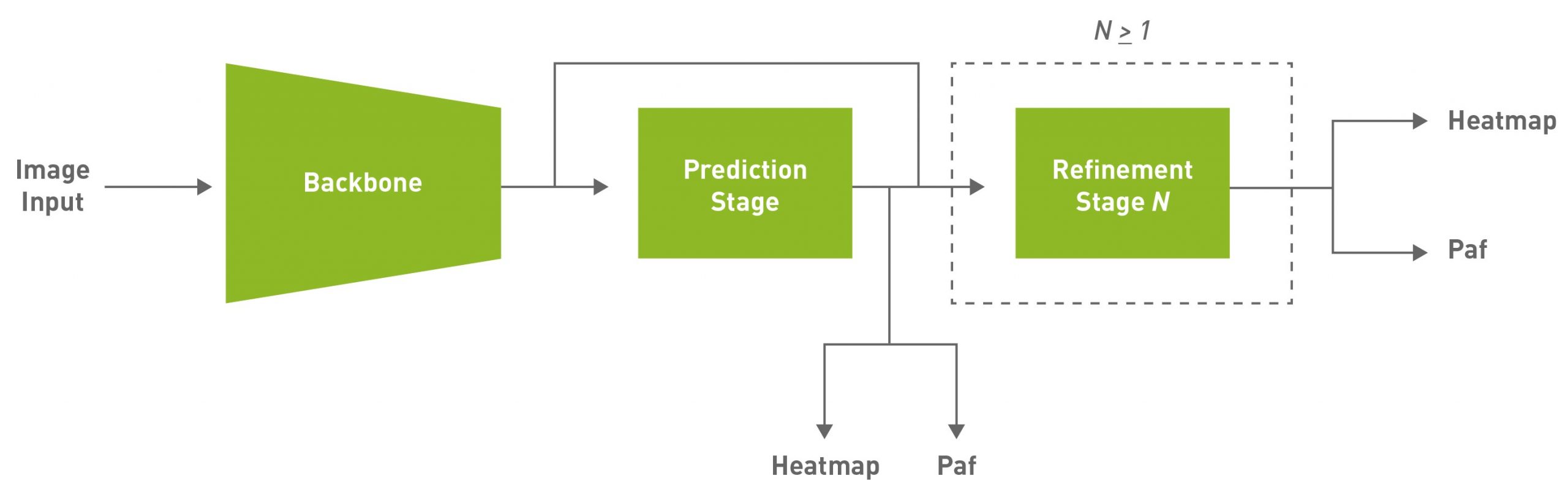
Figure 1 shows that the model architecture includes refinement stages, where each stage refines the results of the previous stage. You can use the stages parameter under the model section to configure this. stages include both the initial prediction stage and the refinement stages. We recommend using a minimum of one refinement stage, and a maximum of six, which corresponds to stages within the range [2, 7].
When you use more stages of refinement, it may help improve the accuracy but keep in mind that this would result in an increased inference time. We use a default of two refinement stages (stages=3) in this post, which is tuned for optimal performance and accuracy. For even faster performance, use stages=2.
Pruning and regularization
Pruning can help with a significant decrease in the number of parameters and maximize speed while preserving the accuracy or at the cost of some drop in accuracy. A higher pruning threshold gives you a smaller model and thus higher inference speed but might cause a drop in accuracy.
The threshold to use depends on the dataset. If the retrain accuracy is good, you can increase this value to get smaller models. Otherwise, lower this value to get better accuracy. We recommend iterating with the prune-retrain cycle until you are satisfied with the accuracy-speed tradeoff. You can also use a higher L1 regularization weight when training the model before pruning. It would push more weights towards zero, making it easier to prune the network weights.
Model accuracy and performance
In this section, we dive deeper into the model accuracy and performance, and compare it against the state of the art, and across platforms.
Comparison with OpenPose
We compare this approach against OpenPose as this method follows a similar single-shot bottom-up methodology. Figure 4 shows that you achieve a much better accuracy-performance tradeoff as compared to the OpenPose model. The accuracy is lower by ~8% AP whereas you achieve close to a 9x speedup for the model trained with the default parameters provided in this post.
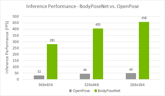
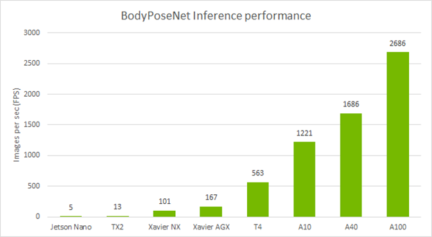
Standalone performance across devices
The following table shows the inference performance of the BodyPoseNet model trained with TLT by using the default parameters. We profiled the model inference with the trtexec command of TensorRT.
Conclusion
In this post, you learned about optimizing body pose models using the BodyPoseNet app in TLT. The post showed taking an open-source COCO dataset with a pretrained backbone from NGC to train and optimize a model with TLT. For information regarding model deployment, see the TLT CV inference pipeline Quick Start Scripts and Deployment instructions.
With this model, you can get up to 9x improvement in inference performance as compared to OpenPose, helping you achieve real-time performance even on embedded devices. Pruning plus INT8 precision gives you the highest inference performance on your edge devices.
For more information, see the following resources:

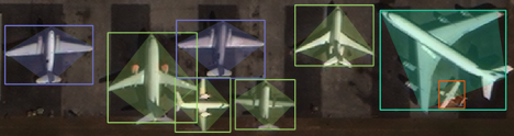
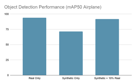
 In AI and computer vision, data acquisition is costly and time-consuming and human-based labeling can be error-prone. The accuracy of the models is also affected by insufficient and poorly balanced data and the prolonged time required to improve the deep learning models. It always requires the reacquisition of data in the real world. The collection, …


 The long, cumbersome slog of data procurement has been slowing down innovation in AI, especially in computer vision, which relies on labeled images and video for training. But now you can jumpstart your machine learning process by quickly generating synthetic data using AI.Reverie. With the AI.Reverie synthetic data platform, you can create the exact training …